Dec 9, 2017 - tic models for Google Home or Google voice search [1]. Room Simulator creates millions of virtual rooms with dif- ferent dimensions and ...
Efficient Implementation of the Room Simulator for Training Deep Neural Network Acoustic Models Chanwoo Kim, Ehsan Variani, Arun Narayanan, and Michiel Bacchiani Google Speech {chanwcom, variani, arunnt, michiel}@google.com
arXiv:1712.03439v1 [cs.SD] 9 Dec 2017
Abstract In this paper, we describe how to efficiently implement an acoustic room simulator to generate large-scale simulated data for training deep neural networks. Even though Google Room Simulator in [1] was shown to be quite effective in reducing the Word Error Rates (WERs) for far-field applications by generating simulated far-field training sets, it requires a very large number of Fast Fourier Transforms (FFTs) of large size. Room Simulator in [1] used approximately 80 percent of Central Processing Unit (CPU) usage in our CPU + Graphics Processing Unit (GPU) training architecture [2]. In this work, we implement an efficient OverLap Addition (OLA) based filtering using the open-source FFTW3 library. Further, we investigate the effects of the Room Impulse Response (RIR) lengths. Experimentally, we conclude that we can cut the tail portions of RIRs whose power is less than 20 dB below the maximum power without sacrificing the speech recognition accuracy. However, we observe that cutting RIR tail more than this threshold harms the speech recognition accuracy for rerecorded test sets. Using these approaches, we were able to reduce CPU usage for the room simulator portion down to 9.69 percent in CPU/GPU training architecture. Profiling result shows that we obtain 22.4 times speed-up on a single machine and 37.3 times speed up on Google’s distributed training infrastructure. Index Terms: Simulated data, room acoustics, robust speech recognition, deep learning
1. Introduction With advancements in deep learning [3, 4, 5, 6, 7, 8], speech recognition accuracy has improved dramatically. Now, speech recognition systems are used not only on portable devices but also on standalone devices for far-field speech recognition. Examples include voice assistant systems such as Amazon Alexa and Google Home [1, 9]. In far-field speech recognition, the impact of noise and reverberation is much larger than near-field cases. Traditional approaches to far-field speech recognition include noise robust feature extraction algorithms [10, 11, 12], on-set enhancement algorithms [13, 14], and multi-microphone approaches [15, 16, 17, 18, 19]. Recently, we observed that training with large-scale noisy data generated by a Room Simulator [1] improves speech recognition accuracy dramatically. This system has been successfully employed for training acoustic models for Google Home or Google voice search [1]. Room Simulator creates millions of virtual rooms with different dimensions and different number of sound sources at different locations and Signal-to-Noise Ratios (SNRs). For every new utterance in the training set, we use a randomly sampled room configuration, so that the same utterance is simulated under different acoustic environments in every epoch during train-
Single Channel Input Batch
Parameter Server (PS) W
∆W
GPU Worker
W ∂L ∂wN
Loss
CPU Room Congifuation Generator
Acoutisc Simulation
.. .
Single or Multi-Channel Simulated Utterance ∂L ∂w1
Feature Extraction
LSTM Stack
f1 , l1
···
LSTM Stack
fN , lN
Training Worker Queue
∂L ∂w1
···
∂L ∂wN
f1 , l1
···
fN , lN
Example Server Queue
Figure 1: Training architecture using cluster of CPUs and GPUs. [2]. Room Simulator is on the CPU side to generate simulated utterances using room configurations. [1]. ing. As will be seen in Sec. 3, if we generate the simulated utterance only once for each input example, the performance is worse. Since different RIRs are applied for the same utterance at every epoch, the intermediate results cannot be cached. Therefore, the noisification process requires very large number of convolution operations. As will be seen in Sec. 3, during training, Room Simulator used up to 80 % of the whole CPU usage if we use the CPU/GPU architecture shown in Fig. 1. In this paper, we describe our approach to reduce the computational portion of the Room Simulator below 10 % of the CPU usage in our CPU/GPU training scheme.
2. Efficient Implementation of the Room Simulation System Fig. 1 shows a high level block diagram of the acoustic model training infrastructure [2]. Since it is not easy to run all the front-end processing blocks such as feature extraction and Voice Activity Detection (VAD) on GPUs, they run on CPUs during training. Even though Fast Fourier Transform (FFT) of the Room Simulator may be efficiently implemented on GPUs, since Room Simulator must feed the simulated utterances to the rest of CPU optimized front-end components, the Room Simulator is also running on CPUs. 2.1. Review of the Room Simulator for Data Augmentation In this section, we briefly review the structure of the Google Room Simulator for generating simulated utterances to train
Figure 2: A simulated room: There may be multiple microphones, a single target sound source, multiple noise sources in a cuboid-shape room with acoustically reflective walls [1].
In our training set used in [1, 9], the average utterance length including non-speech portions marked by the Voice Activity Detector (VAD) is 7.31 s. This corresponds to Nx of 116,991 at 16 kHz. The average length of the RIR in the room simulator used in [1] is 0.243 s, corresponding to the Nh value of 3893. For Google Home the number of noise sources in our training set is 1.55 on average. Thus I is 2.55 including one target source, and J is two, since we use a two-microphones system in [1, 9]. Thus, if we directly use the linear convolution, it requires 2.32 billion multiplications per utterance from (3), which is prohibitively large. Thus, in the “Room Simulator” in [1], we used the frequency domain multiplication using Kiss FFT [24]. To avoid time aliasing, the FFT size N must satisfy N ≥ Nx + M − 1. The j-th microphone channel of the simulated signal yj [n] in (2) is given by: yj [n] =
I−1 X
F F T −1 {F F T {hij [n]} × F F T {xi [n]}} .
i=0
acoustic models for speech recognition systems [1]. We assume a room of a rectangular cuboid-shape as shown in Fig. 2. Assuming that all the walls of a room reflect acoustically uniformly, we use the image method to model the Room Impulse Responses (RIRs) [20, 21, 22, 23]. In the image method, a real room is acoustically mirrored with respect to each wall, which results in grids of virtual rooms. In our work for training the acoustic model for Google Home [1, 9], we consider 17 × 17 × 17 = 4913 virtual rooms for RIR calculation. Following the image method, the impulse response is calculated using the following equation [20, 21]: � �� I−1 gi � X r di fs h[n] = δ n− , di c0 i=0
(1)
where i is the index of each virtual sound source, and di is the distance from that sound source to the microphone, r is the reflection coefficient of the wall, gi is the number of the reflections to that sound source, fs is the sampling rate of the RIR, and c0 is the speed of sound in the air. We use the value of fs = 16, 000 Hz and c0 = 343 m/s for Room Simulator [9]. For di , r, we use numbers created by a random number generator following specified distributions for each impulse response [1]. Assuming that there are I sound sources including one target source and J microphones, the received signal at microphone j is given by: yj [n] =
I−1 X
αij (hij [n] ∗ xi [n]) .
(2)
i=0
Since we used a two-microphones system in [1, 9] J is two, and for the number of noise sources, we used a value from zero up to three with an average of 1.55. Including the target source, the average number of I is 2.55 [1]. 2.2. Efficient Room Impulse Response filtering When the signal and the room impulse response lengths are Nx and Nh respectively, the number of multiplications Ctd required for calculating (2) using the time-domain convolution is given by: Ctd = I × J × Nx × Nh .
(3)
(4) As shown in (4), we perform two FFTs, one IFFT, and one complex element-wise multiplications between two complex spectra for each convolution term in (2). Assuming that radix-2 FFTs are employed, each FFT or IFFT requires N2 log2 (N ) multiplications [25]. In addition, a single element-wise complex multiplication between two complex spectra is required for each convolution term in (2). For real time-domain signals, we need to perform element-wise multiplications for the lower half-spectrum for Discrete Fourier Transform (DFT) indices 0 ≤ k ≤ N/2 since the spectrum has the Hermitian symmetry property [25]. From this discussion, we conclude that the number of real multiplications CFFT for calculating (4) is given by: CFFT = IJ (6N log2 (N ) + 2N ) .
(5)
where N is the FFT size. For the average Nx of 116,991 mentioned above, if we assume that the average N is 217 , (5) requires 69.5 million multiplications per utterance on average. Room Simulator for [1, 9] was implemented in C++ using the Eigen3 linear algebra library [26]. So far we have used the Kiss FFT version of FFT in Eigen3 including acoustic model training for Google Home described in [1, 9]. But, to further speed up frontend computation, we switched from Kiss FFT in Eigen3 to a custom C++ class implementation which internally uses real FFT in FFTW3. A more efficient approach is using the OverLap Add (OLA) FFT filtering [25, 27]. With the OLA FFT filtering, the approximate number of real multiplications is given by: �� � Nx COLA = IJ (4N log2 (N ) + 2N ) N − Nh + 1 � + 2N log2 (N ) , (6) where N is the FFT size, Nx is the length of the entire signal, and Nh is the length of the impulse response. The term 4N log2 (N ) + 2N appears in (6), since there is one FFT, one IFFT, and one element-wise complex multiplication for 0 ≤ k ≤ N/2 for each block. As before, we assumed that each FFT or IFFT requires N2 log2 (N ) multiplications and one jcomplex k Nx multiplication requires four real multiplications in (6). N −M +1 is the number of blocks to process an utterance of length Nx .
Table 1: The profiling result for processing a single utterance using the “Room Simulator” on a local desktop machine Avg. Time per Utterance (ms) Original Room Simulator in [1]
320.8 ms
FFTW3 Real FFT Filtering
44.2 ms
+OLA filtering
19.4 ms
+20 dB RIR cut-off
14.3 ms
(a)
The 2N log2 (N ) term in (6) is required for FFT of the impulse response hij [n]. For the impulse response hij [n], we do not need to repeat it for every block. In our training set consisting of 22 million utterances mentioned above, the average N is 116,991 and the average Nh is 3,893. For this average N and Nh , the minimum value of COLA in (6) is 50.8 millions of real multiplications when N = 214 . The optimal value of N minimizing COLA is different for different Nh and Nx values. For each filtering, we minimize COLA by evaluating this equation with different values of N = 2m where m is an integer.
(b)
Figure 3: The simulated room impulse responses generated in the “Room Simulator” described in Sec. 2: (a) The impulse response without the RIR tail cut-off, (b) with the RIR tail cut-off at 20 dB.
2.3. Room Impulse Response Length Selection The average length of the Room Impulse Response in the original room simulator is estimated to be 3893 samples, which corresponds to 0.243 s. We perform a simple RIR tail-cutoff by finding the RIR power threshold which is η dB below the maximum power of the RIR hij [n]: � η pth = max h2ij [n] × 10− 10 .
(7)
Using pth , we find the cut-off index nc which is the smallest sample index beyond which all the trailing hij [n] has power below the threshold pth : � � � 2 nc = min m max h [n] < pth . (8) m
n>m
Then the final RIR cut-off b hij [n] is given by the following equation: b hij [n] = hij [n],
0 ≤ n ≤ nc + 1.
(9)
Fig. 3 shows the original impulse responses and the corresponding RIR when the cutoff threshold of η is used. To reflect the typical case in our training set, we used the average room dimension, average microphone-to-target distance, and average T60 value among 3 million room configurations described in [1]. As shown in Table 1 and 2, the RIR tail cut-off at 20 dB shows relatively 35.6 % to 69.4 % speed improvement on a local desktop machine and on Google Borg cluster [28]. Fig. 4 shows the profiling results on a local machine with different RIR cutoff thresholds η. The local machine we used has a single Intel(R) Xeon(R) E5-1650 @ 3.20GHz CPU with 6 cores and 32 GB of memory. In Fig. 4, we observe that the computational cost becomes less for the OLA filtering case as we cut the tail portion of the RIR more. For the full FFT case, theoretically, it should remain almost constant regardless of the impulse response length, but due to variation in profiling measurement, there is some small variation.
Figure 4: Profiling result on local desktop machine with different RIR cut-off threshold with and without OverLap Addition FIR filtering.
3. Experimental results In this section, we present speech recognition results and CPU profiling results obtained using Room Simulator with different RIR cut-off thresholds. The acoustic modeling structure to obtain experimental results in this section is somewhat different from those described in [1, 9] for faster training. We use a single-channel 128 log-Mel feature whose window size is 32 ms. The interval between successive frame is 10 ms. The low and upper cutoff frequencies of the Mel filterbank are 125 Hz and 7500 Hz respectively. Since it has been shown that long-duration features represented by overlapping features are helpful [29], four frames are stacked together. Thus we use a context dependent feature consisting of 512 elements given by 128 (the size of the log-mel feature) x 4 (number of stacked frames). This input is down-sampled by a factor of three [30]. The feature is processed by a typical multi-layer Long ShortTerm Memory (LSTM) [31, 32] acoustic model. We use 5-layer LSTMs with 768 units in each layer. The output of the final LSTM layer is passed to a softmax layer. The softmax layer has 8192 nodes corresponding to the number of tied contextdependent phones in our ASR system. The output state label is delayed by five frames, since it was observed that the infor-
Table 2: The CPU usage portion of the FFT and Room Simulator with the respect to the entire CPU pipeline in Fig. 1 and relative speed up on Google Borg cluster [28].
10.11 %
FFTW3 OLA Filter with 20 dB RIR Cut-off 6.23 %
FFTW3 OLA Filter with 10 dB RIR Cut-off 5.08 %
-
34.0 times
57.6 times
59.6 times
80.01 %
13.30 %
9.69 %
8.05 %
-
26.1 times
37.3 times
45.7 times
Original system in [1]
FFTW3 OLA Filter
79.27 %
FFT portion (%) Relative Speed Up in FFT Portion (%) Entire Acoustic Simulation (%) Relative Speed Up in Acoustic Simulation Portion (%)
Table 3: Speech recognition experimental result in terms of Word Error Rates (WERs) with and without MTR using the room simulation system in [1] and different RIR cutoff thresholds.
11.70 % 20.75 % 50.78 % 52.56 % 51.59 % 54.89 %
MTR using One-time Batch Room Simulation 12.07 % 15.58 % 22.47 % 22.39 % 22.12 % 23.42 %
Baseline (On-the-fly Room Simulation) 11.95 % 14.88 % 20.64 % 21.69 % 21.62 % 22.29 %
72.09 %
36.21 %
74.60 %
47.63 %
Baseline without MTR Original Test Set Simulated Noisy Set A Simulated Noisy Set B Device 1 Device 2 Device 3 Device 3 (Noisy Condition) Device 3 (Multi-Talker Condition)
Table 4: Average T60 Time of the Simulated Training Set and Simulated Test Sets A and B.
Average T60 (s)
Simulated
Simulated
Simulated
Training Set
Noisy Set A
Noisy Set B
0.482 s
0.167 s
0.479 s
mation about future frames improves the prediction of the current frame [33, 34]. The acoustic model was trained using the Cross-Entropy (CE) loss as the objective function, using precomputed alignments for utterance as targets. To obtain results in Table 3, we trained for about 45 epochs. For training, we used an anonymized and hand-transcribed 22-million English utterances (18,000-hr) set. The training set is the same as what we used in [1, 9]. For evaluation, we used around 15-hour of utterances (13,795 utterances) obtained from anonymized mobile voice search data. We also generate noisy evaluation sets from this relatively clean voice search data. We use both simulated and rerecorded noisy sets. The average reverberation time in T60 of the simulated training set and two simulated test sets are shown in Table 4. These two simulated test sets are named Simulated Noisy Set A and Simulated Noisy Set B respectively. Since our objective is deploying our speech recognition systems on far-field standalone devices such as Google Home, we rerecorded these evaluation sets using the actual hardware in far-field environment. Note that the actual Google Home hardware has two microphones with microphone spacing of 7.1 cm. In our experiments in this section, we selected the first channel out of two channel data. Three different devices were used in rerecording, and each device was placed in five different loca-
20 dB RIR Cut-off
10 dB RIR Cut-off
5 dB RIR Cut-off
11.43 % 13.96 % 19.58 % 21.35 % 21.26 % 22.86 %
10.75 % 13.59 % 21.37 % 23.20 % 22.90 % 26.47 %
11.20 % 14.99 % 28.27 % 29.53 % 29.39 % 36.71 %
35.88 %
35.83 %
39.99 %
51.11 %
46.03 %
46.21 %
48.36 %
58.31 %
tions in an actual room resembling a real living room. These devices are listed in Table 1 as “Device 1”, “Device 2”, and “Device 3”. As shown in Table 3, we observe that the RIR cutoff up to 20 dB threshold does not adversely affect the performance. However, if we cut the RIR to 5 dB threshold, then the performance under far-field environment becomes significantly worse. This observation also confirms that far-field speech recognition benefits from RIRs with sufficiently long tails in the training set. Table 2 shows how much CPU resource was used when training is done on Google Borg cluster [28] using the CPU/GPU training architecture in Fig. 1. We observe that if we use the FFTW3-based OLA filter using 20 dB RIR cutoff, we may obtain 57.6 times speed-up in the FFT portion. The entire speedup of Room Simulator portion is 37.3 times.
4. Conclusions In this paper, we describe how to efficiently implement an acoustic room simulator to generate large-scale simulated data for training deep neural networks. We implement an efficient OverLap Addition (OLA) based filtering using the open-source FFTW3 library. We investigate into the effects of the Room Impulse Response (RIR) lengths. We conclude that we can cut the tail portions of RIRs whose power is less than 20 dB below the maximum power without sacrificing speech recognition accuracy. However, if we cut off RIR more than that, we observe it adversely affects the performance for reverberant cases. Using the approaches mentioned here, we could reduce the room simulator portion in the CPU usage down to 9.69 % in CPU/GPU training architecture. Profiling result shows that we obtain 22.4 times speed-up on a local desktop machine and 37.3 times speed up on Google Borg cluster.
5. References [1] C. Kim, A. Misra, K.K. Chin, T. Hughes, A. Narayanan, T. Sainath, and M. Bacchiani, “Generation of simulated utterances in virtual rooms to train deep-neural networks for far-field speech recognition in Google Home,” in INTERSPEECH-2017, Aug. 2017, pp. 379–383. [2] E. Variani, T. Bagby, E. McDermott, and M. Bacchiani, “End-toend training of acoustic models for large vocabulary continuous speech recognition with tensorflow,” in INTERSPEECH-2017, 2017, pp. 1641–1645. [Online]. Available: http://dx.doi.org/10. 21437/Interspeech.2017-1284
[17] H. Erdogan, J. R. Hershey, S. Watanabe, M. Mandel, J. Roux, “Improved MVDR Beamforming Using Single-Channel Mask Prediction Networks,” in INTERSPEECH-2016, Sept 2016, pp. 1981–1985. [18] C. Kim and K. K. Chin, “Sound source separation algorithm using phase difference and angle distribution modeling near the target,” in INTERSPEECH-2015, Sept. 2015, pp. 751–755. [19] C. Kim, K. Kumar, B. Raj, and R. M. Stern, “Signal separation for robust speech recognition based on phase difference information obtained in the frequency domain,” in INTERSPEECH-2009, Sept. 2009, pp. 2495–2498.
[3] M. Seltzer, D. Yu, and Y.-Q. Wang, “An investigation of deep neural networks for noise robust speech recognition,” in Int. Conf. Acoust. Speech, and Signal Processing, 2013, pp. 7398–7402.
[20] J. Allen and D. Berkley, “Image method for efficiently simulating small-room acoustics,” J. Acoust. Soc. Am., vol. 65, no. 4, pp. 943–950, April 1979.
[4] D. Yu, M. L. Seltzer, J. Li, J.-T. Huang, and F. Seide, “Feature learning in deep neural networks - studies on speech recognition tasks,” in Proceedings of the International Conference on Learning Representations, 2013.
[21] E. A. Lehmann, A. M. Johansson, and S. Nordholm, “Reverberation-time prediction method for room impulse responses simulated with the image-source model,” in 2007 IEEE Workshop on Applications of Signal Processing to Audio and Acoustics, Oct. 2007, pp. 159–162.
[5] V. Vanhoucke, A. Senior, and M. Z. Mao, “Improving the speed of neural networks on CPUs,” in Deep Learning and Unsupervised Feature Learning NIPS Workshop, 2011.
[22] S. G. McGovern. room impulse response generator. [Online]. Available: https://www.mathworks.com/matlabcentral/ fileexchange/5116-room-impulse-response-generator
[6] G. Hinton, L. Deng, D. Yu, G. E. Dahl, A. Mohamed, N. Jaitly, A. Senior, V. Vanhoucke, P. Nguyen, T. Sainath, and B. Kingsbury, “Deep neural networks for acoustic modeling in speech recognition: The shared views of four research groups,” IEEE Signal Processing Magazine, vol. 29, no. 6, Nov.
[23] ——, “Fast image method for impulse response calculations of box-shaped rooms,” Applied Acoustics, vol. 70, no. 1, pp. 182 – 189, 2009.
[7] T. Sainath, R. J. Weiss, K. W. Wilson, B. Li, A. Narayanan, E. Variani, M. Bacchiani, I. Shafran, A. Senior, K. Chin, A. Misra, and C. Kim, “Multichannel signal processing with deep neural networks for automatic speech recognition,” IEEE/ACM Trans. Audio, Speech, Lang. Process., Feb. 2017. [8] ——, “Raw Multichannel Processing Using Deep Neural Networks,” in New Era for Robust Speech Recognition: Exploiting Deep Learning, S. Watanabe, M. Delcroix, F. Metze, and J. R. Hershey, Ed. Springer, Oct. 2017. [9] B. Li, T. Sainath, A. Narayanan, J. Caroselli, M. Bacchiani, A. Misra, I. Shafran, H. Sak, G. Pundak, K. Chin, K-C Sim, R. Weiss, K. Wilson, E. Variani, C. Kim, O. Siohan, M. Weintraub, E. McDermott, R. Rose, and M. Shannon, “Acoustic modeling for Google Home,” in INTERSPEECH-2017, Aug. 2017, pp. 399– 403. [10] C. Kim and R. M. Stern, “Power-Normalized Cepstral Coefficients (PNCC) for Robust Speech Recognition,” IEEE/ACM Trans. Audio, Speech, Lang. Process., pp. 1315–1329, July 2016. [11] U. H. Yapanel and J. H. L. Hansen, “A new perceptually motivated MVDR-based acoustic front-end (PMVDR) for robust automatic speech recognition,” Speech Communication, vol. 50, no. 2, pp. 142–152, Feb. 2008. [12] C. Kim and R. M. Stern, “Feature extraction for robust speech recognition based on maximizing the sharpness of the power distribution and on power flooring,” in IEEE Int. Conf. on Acoustics, Speech, and Signal Processing, March 2010, pp. 4574–4577.
[24] M. Borgerding, “Kiss fft version https://sourceforge.net/projects/kissfft/, 2010.
1.2.9,”
[25] A. V. Oppenheim and R. W.Scafer, with .J. R. Buck, Discrete-time Signal Processing, 2nd ed. Englewood-Cliffs, NJ: Prentice-Hall, 1998. [26] G. Guennebaud, B. Jacob http://eigen.tuxfamily.org, 2010.
et
al.,
“Eigen
v3,”
[27] R. Crochiere, “A weighted overlap-add method of short-time Fourier analysis/synthesis,” IEEE Trans. Acoust., Speech, and Signal Processing, vol. 28, no. 1, pp. 99–102, feb 1980. [28] A. Verma, L. Pedrosa, M. R. Korupolu, D. Oppenheimer, E. Tune, and J. Wilkes, “Large-scale cluster management at Google with Borg,” in Proceedings of the European Conference on Computer Systems (EuroSys), Bordeaux, France, 2015. [29] H. Sak, A. Senior, K. Rao, and F. Beaufays, “Fast and Accurate Recurrent Neural Network Acoustic Models for Speech Recognition,” in INTERSPEECH-2015, Sept. 2015, pp. 1468–1472. [30] G. Pundak and T. N. Sainath, “Lower Frame Rate Neural Network Acoustic Models,” 2016, pp. 22–26. [Online]. Available: http://dx.doi.org/10.21437/Interspeech.2016-275 [31] S. Hochreiter and J¨urgen Schmidhuber, “Long Short-term Memory,” Neural Computation, no. 9, pp. 1735–1780, Nov. 1997. [32] T. N. Sainath, O. Vinyals, A. Senior, and H. Sak, “Convolutional, long short-term memory, fully connected deep neural networks,” in IEEE Int. Conf. Acoust., Speech and Signal Processing, Apr. 2015, pp. 4580–4584.
[13] ——, “Nonlinear enhancement of onset for robust speech recognition,” in INTERSPEECH-2010, Sept. 2010, pp. 2058–2061.
[33] H. Sak, A. Senior, and F. Beaufays, “Long short-term memory recurrent neural network architectures for large scale acoustic modeling,” in INTERSPEECH-2014, Sept. 2014, pp. 338–342.
[14] C. Kim, K. Chin, M. Bacchiani, and R. M. Stern, “Robust speech recognition using temporal masking and thresholding algorithm,” in INTERSPEECH-2014, Sept. 2014, pp. 2734–2738.
[34] M. Schuster and K. Paliwal, “Bidirectional recurrent neural networks,” IEEE Transactions on Signal Processing, vol. 45, no. 11, pp. 2673–2681, 1997.
[15] T. Nakatani, N. Ito, T. Higuchi, S. Araki, and K. Kinoshita, “Integrating DNN-based and spatial clustering-based mask estimation for robust MVDR beamforming,” in IEEE Int. Conf. Acoust., Speech, Signal Processing, March 2017, pp. 286–290. [16] T. Higuchi and N. Ito and T. Yoshioka and T. Nakatani, “Robust MVDR beamforming using time-frequency masks for online/offline ASR in noise,” in IEEE Int. Conf. Acoust., Speech, Signal Processing, March 2016, pp. 5210–5214.