A novel algorithm for interactive multilabel image/video segmentation is ... the user to specify several free parameters
Efficient Label Propagation for Interactive Image Segmentation Fei Wang Department of Automation, Tsinghua University, Beijing, China
Xin Wang Aplus Company, Beijing, China
Tao Li School of Computer Science, FIU Miami, FL 33199, U.S.A.
[email protected]
[email protected]
[email protected]
Abstract
based algorithms only return the smallest cut separating the seeds (i.e. the labeled pixels), they often produce the small cuts that minimally separate the seeds from the rest pixels when the number seeds is very small, moreover, as the Kway graph cut problem is NP-hard, one often require a use of a heuristic to obtain the final solution. In this paper, we propose a novel interactive image segmentation method called Efficient Label Propagation (ELP), which iteratively propagates the labels of the seeds to the rest unlabeled pixels through the image lattice. Theoretical analysis are presented to guarantee the convergence of the label propagation procedure. Moreover, to increase the efficiency of our approach, we propose a coarse-to-fine scheme to propagate the labels. And the user is allowed to actively adjust the initially labeled seeds according to the segmentation results. We also provide some heuristics that can help the user to achieve satisfactory results with minimum efforts. Finally many experimental results are presented to show the effectiveness of our method. It is worthwhile to highlight the several aspects of our proposed ELP algorithm here:
A novel algorithm for interactive multilabel image/video segmentation is proposed in this paper. Given a small number of pixels with user-defined (or pre-defined) labels, our method can automatically propagate those labels to the remaining unlabeled pixels through an iterative procedure. Theoretical analysis of the convergence property of this algorithm is developed along with the corresponding connections with energy minimization of the Hidden Markov Random Field models. To make the algorithm more efficient, we also derive a multi-level way for propagating the labels. Finally the segmentation results on natural images are presented to show the effectiveness of our method.
1
Introduction
Image segmentation is an integral part of many image processing applications, such as medical images analysis and photo editing. Fully automated segmentation techniques have been constantly improving, however, to the best of the authors’ knowledge, there are rarely any automated image analysis techniques which can be applied autonomously with satisfactory results in general cases. That is why the semi-automated techniques is becoming more and more popular. A semi-automated segmentation algorithm allows the users to participate in the segmentation procedure and give some guidance for the definition of the desired contents to be extracted, so we usually call it interactive segmentation. According to [4], a practical interactive segmentation algorithm must provide four qualities: (1) Fast computation; (2) Fast editing; (3) An ability to produce arbitrary segmentation with enough interactions; (4) Intuitive segmentations. In the last decades, many powerful techniques for interactive image segmentation have been proposed, such as active contour / level set based methods [6][12] and graph cut based methods [1][8][10]. However, despite their success in many situations, there are still a few concerns associated with these algorithms, e.g. it is usually hard to implement the active contour/level set based methods, since they need the user to specify several free parameters; the graph cut
1. Fast computation. Although our algorithm is very similar to random walker in spirit, as we will show later, it is much faster than the random walker method. 2. Fast editing. Due to its iterative nature, our algorithm can perform fast editing by using the previous solution as the initialization of the next propagation. 3. Arbitrary/intuitive segmentation with minimum human efforts. The experiments in this paper show that our algorithm can produce arbitrary/intuitive segmentation through minimum human efforts, which is guaranteed by the active user feedback scheme. So we can see that our algorithm has covered all the qualities that a practical interactive image segmentation algorithm should provide. One issue should be addressed here is that independent of this work, Zhu et al. [15] also proposed a label propagation approach for semi-supervised 1
be the intensity (for gray image) or RGB color (for color image). L = {+1, −1} is the label set1 . yi ∈ L is the label of xi , and Ni is the spatial neighborhood of xi (for computational efficiency, we just use the four-connected neighborhood for each pixel throughout the paper). Then our strategy for propagating the labels can be formulated as: At every iteration step, only the labels of the unlabeled pixels are updated, and the labels of the labeled pixels will be clamped. For an unlabeled pixel xu , its label at iteration t will be computed by X (1) puv yvt−1 , yut =
Figure 1. The graphical model of an image. learning. However, they need the data graph to be completely connected to guarantee the convergence of their algorithm, which is infeasible for large scale applications like image segmentation, since the storage requirement of it is so high. On the contrary, our ELP can work on sparse data graphs, and we also prove the convergence of our algorithm. The rest of this paper is organized as follows. In section 2 we will introduce the original efficient label propagation algorithm together with the theoretical analysis in more detail. Section 3 will present a coarse-to-fine scheme for accelerating our ELP algorithm. Section 4 will illustrate some experimental results of our algorithm on image/vedio segmentation, followed by the conclusions and discussions in section 4.
2
xv ∈Nu
where puv is portion of label information that xu learns P from xv satisfying 0 6 pij 6 1, p = 1. v uv t T Let yt = (y1t , · · · , ylt , · · · , yN ) , and P ∈ RN ×N with its (i, j)-th entry Pij = pij 2 . Since in our label propagation scheme the labels of the labeled pixels will always be clamped, thus we can split y and P as ³ ´T t T t T yt = (yL ) , (yU ) ,
·
PLL PU L
PLU PU U
¸
,
t t where yL and yU correspond to the predicted labels of the labeled and unlabeled pixels. Then we can rewrite Eq.(1) as t t−1 yU = P U L yL + P U U yU ,
Label Propagation on Sparse Grids
(2)
where we have omitted the superscript of yL since it remains the same in all iterations. The final value of each yu can be continuous, and the label of xu can just be determined by the sign of yu . Therefore, the labels of the unlabeled pixels can just be predicted using Eq.(2) iteratively until converged. Now the only problems remained are: (1) how to construct the propagation matrix P; (2) wether the iterative procedure will be converged. In the following two subsections we will investigated these two issues in detail.
In this section we will introduce the basic Label Propagation procedure in detail, together with the theoretical analysis of its convergence property and the relationship with energy minimization of Hidden Markov Random Field.
2.1
P=
Basic Algorithm
The goal of image segmentation is to partition the image pixels into several groups, i.e. assign a proper label to each image pixel. A basic image model is shown in Fig.1, which is composed of two layers. The nodes on different layer correspond to different features of the image pixels. More concretely, the nodes on the top layer (denoted by gray squares) represent the visual features of the pixels, such as intensities and colors; the nodes on the bottom layer (denoted by circles) correspond to the intrinsic features, i.e. labels, of the image pixels. For interactive image segmentation, the user has pre-labeled some of the pixels (denoted by colored squares and circles), and our goal is to label the rest pixels. The basic intuition behind our label propagation method is very simple. First it is an iterative procedure, then at every iteration, each pixel “absorbs” some label information from its spatial neighborhood and updates it own label. And this procedure will be repeated many times until the label of each pixel will not change. Mathematically, let X = {x1 , x2 , · · · , xl , · · · , xN } be the collection of image pixels such that XL = {xi }li=1 is the labeled pixel set and XU = {xu }N u=l+1 is the unlabeled pixel set. xi is the feature vector for pixel i, usually it can
2.2
Constructing the Propagation Matrix
One of the key point for our algorithm to work well is to define a proper propagation matrix P. Intuitively, P should encode the similarities between the pixels, i.e. the more similar xj to xi , the more xi will learn from xj , and the larger Pij will be. To achieve such a goal, we should first define an appropriate similarity function to measure the similarities between pairwise similarities. In image segmentation, such a similarity measure should reflect the change in neighboring pixel intensities or colors. There have been many different similarity functions suggested in [13][14][16]. In this paper, we have preferred (for its simplicity and empirical success) the Gaussian function Wij =
½
¡ ¢ exp −βkxi − xj k2 , 0,
xj ∈ N i , otherwise
(3)
where β > 0 is a free parameter. Eq.(3) has widely been used in many graph-based methods for calculating the edge 1 Let’s consider the two-class problem for the time being, and we will extend our algorithm to multi-class problem in section 2.5. 2 p = 0 for non-neighboring pixel pair (x , x ). ij i j
2
weights [4][7][15]. To make the similarity insensitive to β, W we normalize each Wij as Wij = maxW ij Wij , so that all ij the similarities fall within the range [0,1]. After the construction of W, we can compute the propagation matrix Wij , which satisfies P with its (i, j)-th entry Pij = P W ij j P 0 6 Pij 6 1 and j Pij = 1.
2.3
exist some k such that the k-th row sum of PU U is smaller than 1. Hence according to theorem 3, the spectral radius of PU U is smaller than 1, thus (t)
lim PU U = 0, lim
? yU
2.4
Theorem 2 (H.Minc). Let A be an n × n nonnegative matrix, and λmax is the largest eigenvalue of A, ri 6= 0 (∀i = 1, 2, · · · , n) is the sum of the i-th row of A, then min i
³ Xn
l=1
´ ³ Xn Ail rl /ri 6 r 6 max
l=1
i
Ail rl /ri
´
Theorem 3. Let A be an n × n Markovian matrix, and As is a square matrix of order K derived from A by deleting n − K rows and n − K columns from A, ris is the sum of the i-th row of As , if ∃k, rks 6= 1, λsmax is the maximum eigenvalue of As , then λsmax < 1. Proof. P A is a Markovian matrix means that Aij > 0, j Aij = 1. From theorem 1 we know that the spectral radius of A (i.e. the maximum eigenvalue of A) satisfies ρ(A) 6 1. Since As is a submatrix of A, then according to theorem 2, the spectral radius bound satisfies ´ ³ P n ρ(As ) 6 maxi r1i l=1 Asil rl . Furthermore, for ∀i, l=1
Asil rl /ri
=
(Asi1 r1 + Asi2 r2 + · · · + AsiK rK ) /ri