Efficient MCMC for Gibbs Random Fields using pre-computation arXiv ...

Efficient MCMC for Gibbs Random Fields using pre-computation arXiv:1710.04093v2 [stat.CO] 13 Oct 2017

Aidan Boland1,2 , Nial Friel1,2 , and Florian Maire1,2 1

School of Mathematics and Statistics, University College Dublin 2 Insight Centre for Data Analytics

Abstract Bayesian inference of Gibbs random fields (GRFs) is often referred to as a doubly intractable problem, since the likelihood function is intractable. The exploration of the posterior distribution of such models is typically carried out with a sophisticated Markov chain Monte Carlo (MCMC) method, the exchange algorithm (Murray et al., 2006), which requires simulations from the likelihood function at each iteration. The purpose of this paper is to consider an approach to dramatically reduce this computational overhead. To this end we introduce a novel class of algorithms which use realizations of the GRF model, simulated offline, at locations specified by a grid that spans the parameter space. This strategy speeds up dramatically the posterior inference, as illustrated on several examples. However, using the pre-computed graphs introduces a noise in the MCMC algorithm, which is no longer exact. We study the theoretical behaviour of the resulting approximate MCMC algorithm and derive convergence bounds using a recent theoretical development on approximate MCMC methods.

1

Introduction

The focus of this study is on Bayesian inference of Gibbs random fields (GRFs), a class of models used in many areas of statistics, such as the autologistic model (Besag, 1974) in spatial statistics, the exponential random graph model in social network analysis (Robins et al., 2007), etc. Unfortunately, for all but trivially small graphs, GRFs suffer from intractability of the likelihood function making standard analysis impossible. Such models are often referred to as doubly-intractable in the Bayesian literature, since the normalizing constant of both the likelihood function and the posterior distribution form a source of intractability. In the recent past there has been considerable research activity in designing Bayesian algorithms which overcome this intractability all of which rely on simulation from the intractable likelihood. Such methods include Approximate Bayesian Computation initiated by Pritchard et al. (1999) (see e.g. Marin et al. (2012)

1

for an excellent review) and Pseudo-Marginal algorithms (Andrieu and Roberts, 2009). Perhaps the most popular approach to infer a doubly-intractable posterior distribution is the exchange algorithm (Murray et al., 2006). The exchange algorithm is a Markov chain Monte Carlo (MCMC) method that extends the Metropolis-Hastings (MH) algorithm (Metropolis et al., 1953) to situations where the likelihood is intractable. Compared to MH, the exchange uses a different acceptance probability and this has two main implications: • theoretically: the exchange chain is less efficient than the MH chain, in terms of mixing time and asymptotic variance (see Peskun (1973) and Tierney (1998) for a discussion on the optimality of the MH chain) • computationally: at each iteration, the exchange requires exact and independent draws from the likelihood model at the current state of the Markov chain to calculate the acceptance probability, a step that may substantially impact upon the computational performance of the algorithm For many likelihood models, it is not possible to simulate exactly from the likelihood function. In those situations, Cucala et al. (2009) and Caimo and Friel (2011) replace the exact sampling step in the exchange algorithm with the simulation of an auxiliary Markov chain targeting the likelihood function, whereby inducing a noise process in the main Markov chain. This approximation was extended further by Alquier et al. (2016) who used multiple samples to speed up the convergence of the exchange algorithm. This short literature review of the exchange algorithm and its variants shows that simulations from the likelihood function, either exactly or approximately, is central to those methods. However, this simulation step often compromises their practical implementation, especially for large graph models. Indeed, for a realistic run time, a user may end up with a limited number of draws from the posterior as most of the computational budget is dedicated to obtaining likelihood realizations. In addition, note that since the likelihood draws are conditioned on the Markov chain states, those simulation steps are intrinsically incompatible with parallel computing (Friel et al., 2016). Intuitively, there is a redundance of simulation. Indeed, should the Markov chain return to an area previously visited, simulation of the likelihood is nevertheless carried out as it had never been done before. This is precisely the point we address in this paper. We propose a novel class of algorithms where likelihood realizations are generated and then subsequently re-used at in an online inference phase. More precisely, a regular grid spanning the parameter space is specified and draws from the likelihood at locations given by the vertices of this grid are obtained offline in a parallel fashion. The grid is tailored to the posterior topology using estimators of the gradient and the Hessian matrix to ensure that the pre-computation sampling covers the posterior areas of high probability. However, using realizations of the likelihood at pre-specified grid points instead of at the actual Markov chain state introduces a noise process in the algorithm. This leads us to study the theoretical behaviour of the resulting approximate MCMC algorithm and to derive quantitative convergence bounds using the noisy MCMC framework developed in Alquier et al. (2016). Essentially, our results allow one to quantify how the noise induced by the pre-computing step propagates through to

2

the stationary distribution of the approximate chain. We find an upper bound on the bias between this distribution and the posterior of interest, which depends on the precomputing step parameters i.e. the distance between the grid points and the number of graphs drawn at each grid point. We also show that the bias vanishes asymptotically in the number of simulated graphs at each grid point, regardless of the grid structure. Note that Moores et al. (2015) suggested a similar strategy to speed-up ABC algorithms by learning about the sufficient statistics of simulated data through an estimated mapping function that uses draws from the likelihood function at a pre-defined set of parameter values. This method was shown to be computationally very efficient but its suitability for models with more than one parameter can be questioned. Finally, we note that a related approach has been presented by Everitt et al. (2017) which also relies on previously sampled likelihood draws in order to estimate the intractable ratio of normalising constants. However this approach falls within a sequential Monte Carlo framework. The paper is organised as follows. Section 2 introduces the intractable likelihood that we focus on and details our class of approximate MCMC schemes which uses pre-computed likelihood simulations. We also detail how we automatically specific the grid of parameter values. In Section 3, we establish some theoretical results for noisy MCMC algorithms making use of a pre-computation step. In Section 4, the inference of a number of GRFs is carried out using both pre-computed algorithms and exact algorithms such as the exchange. Results show a dramatic improvement of our method over exact methods in time normalized experiments. Finally, this paper concludes with some related open problems.

2 2.1

Pre-computing Metropolis algorithms Preliminary notation

We frame our analysis in the setting of Gibbs random fields (GRFs) and we denote by y ∈ Y the observed graph. A graph is identified by its adjacency matrix and Y is taken as Y := {0, 1}p×p where p is the number of nodes in the graph. The likelihood function of y is paramaterized by a vector θ ∈ Θ ⊂ Rd and is defined as f (y|θ) =

qθ (y) exp{θT s(y)} = , Z(θ) Z(θ)

where s(y) ∈ S ⊂ Rd+ is a vector of statistics which are sufficient for the likelihood. The normalizing constant, X exp{θT s(y)}, Z(θ) = y∈Y

depends on θ and is intractable for all but trivially small graphs. The aim is to infer the parameters θ through the posterior distribution π(θ | y) ∝

qθ (y) p(θ), Z(θ)

3

where p denotes the prior distribution of θ. In absence of ambiguity, a distribution and its probability density function will share the same notation.

2.2 Computational complexity of MCMC algorithms for doubly intractable distributions In Bayesian statistics, Markov chain Monte Carlo methods (MCMC, see e.g. Gilks et al. (1995) for an introduction) remain the most popular way to explore π. MCMC algorithms proceed by creating a Markov chain whose invariant distribution has a density equal to the posterior distribution. One such algorithm, the Metropolis-Hastings (MH) algorithm Metropolis et al. (1953), creates a Markov chain by sequentially drawing candidate parameters from a proposal distribution θ0 ∼ h( · |θ) and accepting the proposed new parameter θ0 with probability α(θ, θ0 ) := 1 ∧ a(θ, θ0 ) ,

a(θ, θ0 ) :=

qθ0 (y)p(θ0 )h(θ|θ0 ) Z(θ) × . 0 qθ (y)p(θ)h(θ |θ) Z(θ0 )

(1)

This acceptance probability depends on the ratio Z(θ)/Z(θ0 ) of the intractable normalising constants and cannot therefore be calculated in the case of GRFs. As a result, the MH algorithm cannot be implemented to infer GRFs. As detailed in the introduction section, a number of variants of the MH algorithm bypass the need to calculate the ratio Z(θ)/Z(θ0 ), replacing it in Eq. (1) by an unbiased estimator n 1 X qθ (xk ) , x1 , x2 , . . . ∼iid f ( · | θ0 ) . (2) %n (θ, θ0 , x) = n qθ0 (xk ) k=1

Perhaps surprisingly, when n = 1 the resulting algorithm, known as the exchange algorithm (Murray et al., 2006), is π-invariant. The general implementation using n > 1 auxiliary draws was proposed in Alquier et al. (2016) and referred therein as the noisy exchange algorithm. It is not π-invariant but the asymptotic bias in distribution was studied in (Alquier et al., 2016). We note however that when n is large, the resulting algorithm bears little resemblance with the exchange algorithm and really aims at approximating the MH acceptance ratio (1). For clarity, we will therefore refer to the exchange algorithm whenever n = 1 draw of the likelihood is needed at each iteration and to the noisy Metropolis-Hastings whenever n > 1. From Eq. (2), we see that those modified MH algorithms crucially rely on the ability to sample efficiently from the likelihood distribution (X ∼ f ( · | θ) for any θ ∈ Θ). While perfect sampling is possible for certain GRFs, for example for the Ising model (Propp and Wilson, 1996), it can be computationally expensive in some cases, including large Ising graphs. For some GRFs such as the exponential random graph model, perfect sampling does not even exist yet. Cucala et al. (2009) and Caimo and Friel (2011) substituted the iid sampling in Eq. (2) with n = 1 draw from a long auxiliary Markov chain that admits f ( · | θ) as stationary distribution. Convergence of this type of approximate exchange algorithm was studied in Everitt (2012) under certain assumptions on the main Markov chain. The computational bottleneck of those methods is clearly the simulation step, a drawback which is amplified when n is large and inference is on high-dimensional data such as large graphs.

4

Intuitively, obtaining a likelihood sample at each step independently of the past history of the chain seems to be an inefficient strategy. Indeed, the Markov chain may return to areas of the state space previously visited. As a result, realizations from the likelihood function are simulated at similar parameter values multiple times, throughout the algorithm. Under general assumptions on the likelihood function, data simulated at similar parameter values will share similar statistical features. Hence, repeated sampling without accounting for previous likelihood simulations seems to lead to an inefficient use of computational time. However, the price to pay to use information from the past history of the chain to speed up the simulation step is the loss of the Markovian dynamic of the chain, leading to a so-called adaptive Markov chain (see e.g. Andrieu and Thoms (2008)). We do not pursue this approach in this paper, essentially since convergence results for adaptive Markov chains depart significantly from the theoretical arguments supporting the validity of the exchange and its variants. In a different context, Moores et al. (2015) addressed the computational expense of repeated simulations of Gibbs random fields used within an Approximate Bayesian Computation algorithm (ABC). The authors defined a pre-processing step designed to learn about the distribution of the summary statistics of simulated data. Part of the total computational budget is spent offline, simulating data from parameter values across the parameter space Θ. Those pre-simulated data are interpolated to create a mapping function Θ → S that is then used during the course of the ABC algorithm to assign an (estimated) sufficient statistics vector to any parameter θ for which simulation would be otherwise needed. Moores et al. (2015) examined a particular GRF, the single parameter hidden Potts model. They combined the pre-processing idea with path sampling (Gelman and Meng, 1998) to estimate the ratio of intractable normalising constants. The method presented in Moores et al. (2015) is suitable for single parameter models but the interpolation step remains a challenge when the dimension of the parameter space is greater than 1. Inspired by the efficiency of a pre-computation step, we develop a novel class of MCMC algorithms, Pre-computing Metropolis-Hastings, which uses pre-computed data simulated offline to estimate each normalizing constant ratio Z(θ)/Z(θ0 ) in Eq. (1). This makes the extension to multi-parameter models straightforward. The steps undertaken during the pre-computing stage are now outlined.

2.3

Pre-computation step

Firstly, a set of parameter values, referred to as a grid, G := (θ˙1 , ..., θ˙M ) must be chosen from which to sample graphs from. G should cover the full state space and especially the areas of high probability of π. Finding areas of high probability is not straightforward as this requires knowledge of the posterior distribution. Fortunately, for GRFs we can use Monte Carlo methods to obtain estimates of the gradient and the Hessian matrix of the log posterior at different values of the parameters, which will allow to build a meaningful grid. For a GRF, the well known identity ∇θ log π(θ|y) = s(y) − Ef ( · | θ) s(X) + ∇θ log p(θ)

5

allows the derivation of the following unbiased estimate of the gradient of the log posterior at a parameter θ ∈ Θ: G(θ, y) := s(y) −

N 1 X s(Xi ) + ∇θ log p(θ) , N

X1 , X2 . . . ∼iid f ( · | θ).

(3)

i=1

Similarly, the Hessian matrix of the log posterior at a parameter θ ∈ Θ can be unbiasedly estimated by: N

1 X H(θ) := {s(Xi ) − s¯} {s(Xi ) − s¯}T + ∇2 log p(θ) , N −1 i=1

X1 , X2 . . . ∼iid f ( · | θ) , (4) where s¯ is the average vector of simulated sufficient statistics. The grid specification begins by estimating the mode of the posterior θ∗ . This is achieved by mean of a stochastic approximation algorithm (e.g. the Robbins-Monro algorithm (Robbins and Monro, 1951)), using the log posterior gradient estimate G defined at Eq. (3). The second step is to estimate the Hessian matrix of the log posterior at θ∗ using Eq. (4), in order to get an insight of the posterior curvature at the mode. We denote by V := [v1 , . . . , vd ] the matrix whose columns are the eigenvectors vi of the inverse Hessian at the mode and by Λ := diag(λ1 , . . . , λd ) the diagonal matrix filled with its eigenvalues. The idea is to construct a grid that preserves the correlations between the variables. It is achieved by taking regular steps in the uncorrelated space i.e. the space spanned by [v1 , . . . , vn ], starting from θ∗ and until subsequent estimated gradients are close to each other. The idea is that, for regular models, once the estimated gradients of two successive parameters are similar, the grid has hit the posterior distribution support boundary. Two tuning parameters are required: a threshold parameter for the gradient comparison m > 0 and an exploratory magnitude parameter ε > 0. The grid specification is rigorously outlined in Algorithm 1. Note that in Algorithm 1, we have used the notation δj for the d-dimensional indicator vector of direction j i.e. {δj }` = 1j=` The left panel of Figure 1 shows an example of a naively chosen grid built following standard coordinate directions for a two dimensional posterior distribution. The grid on the right hand side is adapted to the topology of the posterior distribution as described above. This method can be extended to higher dimensional models, but the number of sample grid points would then increase exponentially with dimension. In this paper we do not look beyond two dimensions. Hereafter, we denote by {θ˙m , m ≤ M } the parameters constituting the grid G, assuming M grid points in total. The second step of the pre-computing step is to 1 , ..., X n ) from the likelihood sample for each θ˙m ∈ G, n iid random variables (Xm m function f ( · |θ˙m ). Note that this step is easily parallelised and samples can therefore be obtained from several grid points simultaneously. Parallel processing can be used to reduce considerably the time taken to sample from every pre-computed grid value. Essentially, these draws allow to form unbiased estimators for any ratio of the type

6

Algorithm 1 Grid specification 1: require θ ∗ , V , Λ, m and ε. 2: Initialise the grid with G = {θ ∗ } 3: for i ∈ {1, . . . , d} do 4: for all θ ∈ G do 5: Set j = 0 and θ0 = θ 6: Calculate θ˜ = θ0 + εV Λ1/2 δi ˜ − G(θj )k > m do 7: while kG(θ) 8: Set j = j + 1, θj = θ˜ and G = G ∪ {θj } 9: Calculate θ˜ = θj + εV Λ1/2 δi 10: end while 11: end for 12: end for 13: Obtain a second grid G0 by repeating steps (2)–(12), but moving in the negative direction i.e. θ˜ = θ − εV Λ1/2 δi . 14: return G = G ∪ G0

θ2

θ2

θ1

θ1

Figure 1: Example of a naive (left panel) and informed (right) grid for a two dimensional posterior distribution. The informed grid was obtained using the process described in Algorithm 1.

7

Z(θ)/Z(θ˙m ): n n k) \ Z(θ) 1X 1 X qθ (Xm k = := exp(θ − θ˙m )T s(Xm ). k) ˙ n n q (X Z(θm ) n ˙m m θ k=1 k=1

(5)

Note that those estimators depend on the simulated data only through the sufficient k ). As a consequence, only the sufficient statistics S := {sk } statistics skm := s(Xm m m,k need to be saved, as opposed to the actual collection of simulated graphs at each grid point. In the following we denote by U := {S, G} the collection of the pre-computing data comprising of the grid G and the simulated sufficient statistics S.

2.4

Estimators of the ratio of normalising constants

We now detail several pre-computing version of the Metropolis-Hastings algorithm. The central idea is to replace the ratio of normalizing constants in the MetropolisHastings acceptance probability (1) by an estimator based on U. As a starting point ˙ ∈ Θ3 , this can be done by observing that for all (θ, θ0 , θ)  ˙ Z(θ) Z(θ) Z(θ) Z(θ0 ) Z(θ) = = , (6) ˙ Z(θ0 ) ˙ ˙ Z(θ0 ) Z(θ) Z(θ) Z(θ) and in particular for any grid point θ˙ ∈ G. We thus consider a general class of estimators of Z(θ)/Z(θ0 ) written as 0 ρX n (θ, θ , U) :=

0 ΨX n (θ, θ , U) , 0 ΦX n (θ, θ , U)

(7)

where Ψn and Φn are unbiased estimators of the numerator and the denominator of the right hand side of (6), respectively, based on U. In (7), X simply denotes the different type of estimators considered. To simplify notations and in absence of ambiguity, the dependence of ρn , Ψn and Φn on θ, θ0 , U and X is made implicit and we stress that given (θ, θ0 , U, X), the estimators Ψn and Φn are deterministic. We first note that ρn as defined in (7) is not an unbiased estimator of Z(θ)/Z(θ0 ). In fact, resorting to biased estimators of the normalizing constants ratio is the price to pay for using the pre-computed data. This represents a significant departure compared to the algorithms designed in the noisy MCMC literature (Alquier et al., 2016; MedinaAguayo et al., 2016). Nevertheless, as we shall see in the next Section, this does not prevent us from controlling the distance between the distribution of the pre-computing Markov chain and π. We propose a number of different estimators of Ψn and Φn . Those estimators share in common the idea that, given the current chain location θ and an attempted move θ0 , a path of grid point(s) {θ˙τ1 , θ˙τ2 , . . . , θ˙τC } ⊂ G connects θ to θ0 . The simplest path consists of the singleton {θ˙τ }, where θ˙τ is any grid point. Since only one grid point is used, we refer to this estimator as the One Pivot estimator. Following (6), the estimators Ψn and Φn are defined as P  OP Ψn (θ, θ0 , U) := 1/n nk=1 qθ (Xτk )/qθ˙τ (Xτk ) , P (8) n 0 k k ΦOP n (θ, θ , U) := 1/n k=1 qθ0 (Xτ )/qθ˙τ (Xτ ) .

8

However, for some (θ, θ0 , θ˙τ ) ∈ Θ2 × G, the variance of Ψn or Φn defined in Eq. (8) may be large. This is especially likely when kθ − θ˙τ k  1 or kθ0 − θ˙τ k  1. The following Example illustrates this situation. Example 1. Consider the Erd¨ os-Renyi graph model, where all graphs y ∈ Y with the same number of edges s(y) are equally likely. More precisely, the dyads are independent and connected with a probability %(θ) := logit−1 (θ) for any θ ∈ R. The likelihood function is given for any θ ∈ R by f (y | θ) ∝ exp{θs(y)}. For this model, the
normalizing p p ¯ constant is tractable. In particular, Z(θ) = {1 + exp(θ)} where p¯ = 2 and p is the number of nodes in the graph. For all θ ∈ R, consider estimating the ratio Z(θ0 )/Z(θ) with θ0 = θ + h for some h > 0 using the estimator n n \ Z(θ + h) 1 X qθ+h (Xk ) 1X = exp{hs(Xk )} , Xk ∼iid f ( · | θ) . = Z(θ) n qθ (Xk ) n n

k=1

k=1

Then, when h increases, the variance vn of this estimator diverges exponentially i.e. nvn (h) ∼ exp(2h¯ p)ν(θ) ,

(9)

where ∼ denotes here the asymptotic equivalence notation and ν(θ) = %(θ)p¯(1 − %(θ)p¯) is a constant. Remarkably, ν(θ) can be interpreted as the variance of the Bernoulli trial with the full graph and its complementary event as outcomes. Proof. By straightforward algebra, we have   1 1 + exp(2h + θ) p¯ vn (h) = {1 − R(θ, h)} , n 1 + exp(θ) where R(θ, h) =

{1 + exp(θ + h)}2¯p . {1 + exp(2h + θ)}p¯ {1 + exp(θ)}p¯

Asymptotically in h, we have R(θ, h) ∼

exp(¯ pθ) p¯ p¯ = %(θ) {1 + exp(θ)}

and noting that   exp{¯ pθ} 1 + exp(2h + θ) p¯ ∼ exp(2h¯ p) = exp(2h¯ p)%(θ)p¯ 1 + exp(θ) {1 + exp(θ)}p¯ concludes the proof. This is a concern since as we shall see in the next Section, the noise introduced by the pre-computing step in the Markov chain is intimately related to the variance of the estimator of Z(θ)/Z(θ0 ). In particular, the distance between the pre-computing chain distribution and π can only be controlled when the variance of Ψn and Φn is bounded. Example 1 shows that this is not necessarily the case, for some Gibbs random fields at least. The following Proposition hints at the possibility to control the variance of Ψn and Φn when kθ − θ0 k  1.

9

Proposition 1. For any Gibbs random field model and all (θ, θ0 ) ∈ Θ2 , the variance of the normalizing constant estimator n d Z(θ) 1 X qθ (Xk ) := , Xk ∼iid f ( · | θ0 ) Z(θ0 ) n qθ0 (Xk ) n

k=1

decreases when kθ − θ0 k ↓ 0 and more precisely d Z(θ) var = O(kθ − θ0 k2 ) . Z(θ0 )

(10)

n

Proposition 1 motivates the consideration of estimators that may have smaller variability than the One Pivot estimator. (1) Direct Path estimator: the path between θ and θ0 consists now of two grid points {θ˙1 , θ˙2 } defined such that θ˙1 = arg minθ∈G kθ˙ − θk and θ˙2 = arg minθ∈G kθ˙ − θ0 k. ˙ ˙ We therefore extend (6) and write  Z(θ) Z(θ) Z(θ˙1 ) Z(θ˙2 ) Z(θ) Z(θ˙1 ) Z(θ0 ) = = . Z(θ0 ) Z(θ˙1 ) Z(θ˙2 ) Z(θ0 ) Z(θ˙1 ) Z(θ˙2 ) Z(θ˙2 ) This leads to two estimators Ψn and Φn defined as P P  DP Ψn (θ, θ0 , U) := 1/n nk=1 qθ (X1k )/qθ˙1 (X1k ) × 1/n nk=1 qθ˙1 (Xk2 )/qθ˙2 (Xk2 ) , Pn k k 0 ΦDP n (θ, θ , U) := 1/n k=1 qθ0 (X2 )/qθ˙2 (X2 ) . (11) (2) Full Path estimator: the path between θ and θ0 consists now of adjacent grid points p(θ, θ0 ) := {θ˙1 , θ˙2 , . . . , θ˙C }, where C > 1 is a number that depends on θ and θ0 . Note that given (θ, θ0 ), there is not only one path such as p connecting θ to θ0 . However, for any possible path, two adjacent points {θ˙i , θ˙i+1 } ⊂ p(θ, θ0 ) always satisfy the following identity (in the basis given by the eigenvector of H(θ∗ )):   ∃ j ∈ {1, . . . , d} , V T θ˙i − θ˙i+1 = ±εδj , where δj refers to the d-dimensional indicator vector of direction j i.e. {δj }` = 1j=` . As before, we extend (6) to accommodate this situation and write  Z(θ) Z(θ) Z(θ˙1 ) Z(θ˙C−1 ) Z(θ˙C ) Z(θ) Z(θ˙1 ) Z(θ˙C−1 ) Z(θ0 ) = = ×· · ·× ×· · ·× . Z(θ0 ) Z(θ˙1 ) Z(θ˙2 ) Z(θ˙C ) Z(θ0 ) Z(θ˙1 ) Z(θ˙2 ) Z(θ˙C ) Z(θ˙c ) This then lead to consider two estimators Ψn and Φn defined as  Pn Pn FP 0 k k × 1/n 2 2   Ψn (θ, θ , U) := 1/n k=1 qθ (X1 )/qθ˙1 (X1 ) P k=1 qθ˙1 (Xk )/qθ˙2 (Xk ) k × · · · × 1/n nk=1 qθ˙C−1 (XC−1 )/qθ˙C (XCk ) , P   ΦFP (θ, θ0 , U) := 1/n n q 0 (X k )/q (X k ) . n k=1 θ C C θ˙C (12)

10

Variants of the Direct Path and Full Path estimators exist. For the Direct Path, Ψn could be estimating Z(θ)/Z(θ˙τ1 ) and Φn the ratio Z(θ˙θ0 )/Z(θτ1 ). For the Full Path, defining θ˙τm as a middle point of p(θ, θ0 ), Φn and Ψn could respectively be defined as estimators of Z(θ)/Z(θ˙τm ) and Z(θ0 )/Z(θ˙τm ) using the same number of grid points in both estimators. However, our experiments have shown that these alternative estimators have very similar behaviour with those defined in Eqs. (11) and (12). In particular, the variance of an estimator does not vary much when path points are removed from the numerator estimator and added to the denominator estimator, or conversely. As hinted by Proposition 1, the discriminant feature between those estimators is the distance between grid points constituting the path. In this respect, the variance of the Full Path estimator was always found to be lower than that of the Direct Path or One Pivot estimators. Even though establishing a rigorous comparison result between those estimators is a challenge on its own, a reader might be interested in the following result that somewhat formalizes our empirical observations. Proposition 2. Let (θ, θ0 ) ∈ Θ and consider the Direct Path and Full Path estimators of Z(θ)/Z(θ0 ) defined at (11) and (12). Denoting by {θ˙1 , . . . , θ˙C } a full path connecting θ to θ0 , we define for i ∈ {2, . . . , C} Rni as the estimator of Z(θ˙i−1 )/Z(θ˙i ) and Rn2C as the estimator of Z(θ˙1 )/Z(θ˙C ) i.e. Rni

k n 1 X qθ˙i−1 (Xi ) , = n qθ˙ (Xik ) k=1

Rn2C

n k 1 X qθ˙1 (XC ) = , n qθ˙ (XCk ) k=1

i

Xik ∼iid f ( · | θ˙i ) .

(13)

C

Let vnFP and vnDP be the variance of the Full Path and Direct Path estimators using n pre-computed sufficient statistics are drawn at each grid point. Assume Φn and Ψn are independent. Then, there exists a positive constant γ < ∞ such that  vnDP − vnFP = γ var(Rn2C ) − var(Rn2 × · · · × RnC ) . (14) Moreover, n o 1 var exp (θ˙1 − θ˙C )T s(XC ) n and for large n and C and small ε we have var(Rn2C ) =

var(Rn2

× ··· ×

RnC )

)2 ( C
ε4 X Z(θ˙i )Z(θ˙1 ) = vi + o ε4 /n , n Z(θ˙i−1 )Z(θ˙C ) i=2

(15)

(16)

where {v1 , v2 , . . .} is a sequence of finite numbers such that vi ∈ O(ε). Proposition 2 shows that for a large enough number of pre-computed draws n, a long enough path and a dense grid i.e.   1, the variance of the Full Path estimator is several order of magnitude less than that of the Direct Path estimator. In particular, unlike the Full Path estimator, the grid refinement does not help to reduce the variance of the Direct Path estimator. Proposition 2 coupled with the observation made at Example 1 helps to understand the variance reduction achieved with the Full Path estimator compared to the Direct Path estimator.

11

θ2

θ2 θ˙τC

θ˙τ2 θ˙τ

θ0

θ0 θ

θ˙τ1

θ

θ˙τ1

θ1

θ1

Figure 2: Example of paths between two parameters (θ, θ0 ) in a two-dimensional space Θ. The solid black lines represent level lines of the target distribution and the black dots represent the grid vertices G = {θ˙1 , . . . , θ˙M }. The thick lines show the paths p(θ, θ0 ) used by the different estimators introduced in Eqs. (8), (11), (12): an example of a One Pivot path ˙ (blue) and a Direct Path p(θ, θ0 ) = {θ˙1 , θ˙2 } (red) are shown on the left panel. p(θ, θ0 ) = {θ} Two examples of Full Paths p(θ, θ0 ) = {θ˙1 , . . . , θ˙C } (red) are illustrated on the right panel: multiple possible full paths between θ and θ0 could be used to average a number of Full Path estimators. Note that when the parameter space is two-dimensional or higher, there is more than one choice of path connecting θ to θ0 . The right panel of Figure 2 shows two different paths. In this situation, one could simply average the Full Path estimators obtained through each (or a number of) possible path. The different steps included in the Pre-computing Metropolis algorithm are summarized in Algorithm 2.

3 Asymptotic analysis of the pre-computing Metropolis-Hastings algorithms In this section, we investigate the theoretical guarantees for the convergence of the Markov chain {θk , k ∈ N} produced by the pre-computing Metropolis algorithm (Alg. 2) to the posterior distribution π. The Markov transition kernels considered in this section are conditional probability distributions on the measurable space (Θ, ϑ) where ϑ is the σ-algebra taken as the Borel set on Θ. We will use the following transition kernels:

12

Algorithm 2 Pre-computing Metropolis algorithm (1)-Pre-computing Require: Grid refinement parameter ε > 0 and number of draws n ∈ N 1: Apply Algorithm 1 to define the grid G = {θ˙1 , . . . , θ˙M }. 2: Initiate the collection of sufficient statistics to S = {∅}. 3: for m = 1 to M do 4: for k = 1 to n do k 5: Draw Xm ∼iid f (· | θ˙j ) k 6: Calculate the vector of sufficient statistics skm = s(Xm ) 7: Append the pre-computed sufficient statistics set S = {S ∪ skm } 8: end for 9: end for Return: The pre-computed data U = {G, S} (2)-MCMC sampling Require: Initial distribution µ and proposal kernel h, pre-computed data U and a type of estimator ρX n , X ∈ {OP, DP, FP} 1: Initiate the Markov chain with θ0 ∼ µ 2: Identify the closest grid point from θ0 , say θ˙i , and calculate n

n o 1X T k ˙ exp (θ0 − θi ) si . Z0 := n k=1 for i = 1, 2, . . . do 4: Draw θ0 ∼ h( · | θi−1 ) 5: Identify the closest grid point from θ0 , say θ˙i , and calculate

3:

n

n o 1X 0 T k ˙ exp (θ − θi ) si . Z := n k=1 0

Using Zi−1 , Z 0 and S, calculate the normalizing ratio estimator ρX n , depending on the type of estimator X using Eq. (8), (11) or (12). 7: Set θi = θ0 and Zi = Z 0 with probability 6:

α ¯ (θi−1 , θ0 , U) := 1 ∧ a ¯(θi−1 , θ0 , U) , a ¯(θi−1 , θ0 , U) = and else set θi = θi−1 and Zi = Zi−1 . end for Return: The Markov chain {θ1 , θ2 , . . .}. 8:

13

qθ0 (y)p(θ0 )h(θi |θ0 ) 0 × ρX n (θi−1 , θ , U) (17) qθi (y)p(θi )h(θ0 |θi )

• Let P be the Metropolis-Hastings (MH) transition kernel defined as: Z h(dθ0 | θ)α(θ, θ0 ) + δθ (A)r(θ) , P (θ, A) = A Z r(θ) = 1 − h(dθ0 | θ)α(θ, θ0 ) , (18) Θ

where δθ is the dirac mass at θ and α the (intractable) MH acceptance probability defined at Eq. (1). • Let P¯U be the pre-computing Metropolis transition kernel, conditioned on the pre-computing data U and defined as: Z h(dθ0 | θ)α ¯ (θ, θ0 , U) + δθ (A)¯ r(θ, S) , P¯U (θ, A) = A Z r¯(θ, U) = 1 − h(dθ0 | θ)¯ α(θ, θ0 , U) , (19) Θ

where α ¯ is the pre-computing Metropolis acceptance probability defined at Eq. (17). We recall that the MH Markov chain is π-invariant, a property which is lost by the pre-computing Metropolis algorithm. In what follows, we regard P¯ as a noisy version of the MH kernel P and α ¯ as an approximation of the intractable quantity α. In terms of notations, we will use the following: for any i ∈ N, P i is the transition kernel P iterated i times and for anyR measure µ on (Θ, ϑ), µP is the probability measure on (Θ, ϑ) defined as µP (A) := µ(dθ)P (θ, A). Using the theoretical framework, developed in Alquier et al. (2016), we show that under certain assumptions, the distance between the distribution of the pre-computing Metropolis Markov chain and π can be made arbitrarily small, in function of the grid refinement and the number of auxiliary draws. The metric used on the space of probability distributions is the total variation distance, defined for two distributions (ν, µ) that admit a density function with respect to the Lebesgue measure as Z kν − µk := (1/2) |ν(θ) − µ(θ)|dθ . Θ

3.1

Noisy Metropolis-Hastings

We first recall the main result from Alquier et al. (2016) that will be used to analyse the pre-computing Metropolis algorithm. Proposition 3 (Corollary 2.3 in Alquier et al. (2016)). Let us assume that, • (H1) A MH Markov chain with transition kernel P (Eq. 18), proposal kernel h and acceptance probability α (Eq. 1) is uniformly ergodic i.e. there are constants B > 0 and ρ < 1 such that ∀i ∈ N,

sup kδθ0 P i − πk ≤ Bρi .

θ0 ∈Θ

14

• (H2) There exists an approximation of the Metropolis acceptance ratio a, a ˆ(θ, θ0 , X) that satisfies for all (θ, θ0 ) ∈ Θ2 ˆ(θ, θ0 , X) − a(θ, θ0 ) ≤ (θ, θ0 ) , E a where the expectation is with respect to the noise random variable X. Then, denoting by Pˆ the noisy Metropolis-Hastings kernel (Eq. 19), we have for any starting point θ0 ∈ Θ and any integer i ∈ N:   Z Bρλ i i ˆ kδθ0 P − δθ0 P k ≤ λ − sup dθ0 h(θ0 |θ)(θ, θ0 ) , (20) 1 − ρ θ∈Θ   log(1/B) . where λ = log(ρ)

An immediate consequence of Proposition 3 is that if  is uniformly bounded, i.e. there exists some ¯ > 0 such that for all (θ, θ0 ) ∈ Θ2 , (θ, θ0 ) ≤ ¯ < ∞, then   Bρλ i i ˆ ∀i ∈ N, kδθ0 P − δθ0 P k ≤ ¯ λ − . (21) 1−ρ Moreover, defining π ˆi as the distribution of the i-th state of the noisy chain yields   Bρλ lim kπ − π ˆi k ≤ ¯ λ − . (22) i→∞ 1−ρ

3.2 Convergence of the pre-computing Metropolis algorithm In preparation to apply Proposition 3, we make the following assumptions: • (A1) there is a constant cp such that for all θ ∈ Θ, 1/cp ≤ p(θ) ≤ cp . • (A2) there is a constant ch such that for all (θ, θ0 ) ∈ Θ2 , 1/ch ≤ h(θ0 |θ) ≤ ch . Assumptions (A1) and (A2) are typically satisfied when Θ is a bounded set and p and h( · | θ) are dominated by the Lebesgue measure. Under similar assumptions, Proposition 3 was applied to the noisy Metropolis algorithm (Alquier et al., 2016) that uses the unbiased estimator %n (Eq. 2). More precisely, it was shown that the distance √ between π and π ˆi satisfies kπ − π ˆi k ≤ κ/ n, where κ > 0 is a positive constant, asymptotically in i. Establishing an equivalent result for the pre-computing Metropolis algorithms is not straightforward. The main difficulty is that the acceptance ratio a ˜(θ, θ0 , U) (Eq. 17) is a 0 biased estimator of the MH acceptance ratio a(θ, θ ) (Eq. 1). The following Proposition only applies to the pre-computing Metropolis algorithm involving the approximation of the normalizing constant ratio using the full path estimator. Weaker results can be obtained using similar arguments for the One Pivot and Direct Path estimators.

15

Proposition 4. Assume that (H1), (A1) and (A2) hold and for any (θ, θ0 ) ∈ Θ2 define by C the shortest path p(θ, θ0 ) length. Then, there exists a sequence of functions un : N → R+ and a function v : R+ → R+ satisfying √ p C v(ε) = 2 dψ1 ε + o(ε1/2 ) , (23) un (C) = √ + o(n−1/2 ) , n such that the pre-computing Metropolis acceptance ratio a ¯(θ, θ0 , S) (Eq. 17) satisfies E a ¯(θ, θ0 , S) − a(θ, θ0 ) ≤ 2c2p c2h K1 K2C+2d−1 (ε) {un (C) + v(ε)} . (24) In Eq. (23), ψ1 < ∞ is a constant, n is the number of pre-computed GRF realizations for each grid point and ε is the distance between grid points. In Eq. (24), K1 and K2 () are finite constants such that K2 () → 1 when  ↓ 0. Corollary 1. Define by π ¯i the distribution of the i-th iteration of the pre-computing Metropolis algorithm implemented with the Full Path estimator. Under Assumptions (H1), (A1) and (A2), we have lim kπ − π ¯i k ≤ κ ¯ K22d−1 (ε)

i→∞

M X

K2c (ε) {un (c) + v(ε)} pc ,

(25)

c=1

where pc = P{C = c} is the probability distribution of the path length and   Bρλ κ ¯ = λ− 2c2p c2h K1 . 1−ρ In Eq. (25), un and v are defined in Eq. (23). Corollary 1 states that the asymptotic distance between the pre-computing Markov chain distribution and π admits an upper bound that has two main components: p • un (c) ∼ c/n which is related to the variance of each estimator of a normalizing constant ratio estimator, √ • v(ε) ∼ 2 dψ1 ε that arises from using a fixed step size grid. This provides useful guidance as to how to tune the pre-computing parameters n and ε. In particular, n should increase with the proposal kernel h variance and ε should decrease with the dimension of Θ, that is d. When ε → 0 the upper bound of kπ − π ¯i k √ is in 1/ n which is in line with the noisy Metropolis rate of (Alquier et al., 2016). Interestingly, when ε  1, we believe that our bound is tighter thanks to the lower variability of the Full Path estimator compared to the unbiased estimator %n (Eq. 2) √ used in the noisy Metropolis algorithm. Indeed, their bound is in o(K14 / n) which, √ given the crude definition of K1 , is much looser compared to our o(K1 / n) bound. The following Proposition shows that when the number of data n simulated at the pre-computing step tends to infinity then E |¯ a(θ, θ0 , S) − a(θ, θ0 )| vanishes. This result is somewhat reassuring as it suggests that the pre-computing algorithm will converge to the true distribution, asymptotically in n, regardless of the grid specification. However, it is not possible to embed this result in the framework developed in Alquier et al. (2016) as the convergence comes without a rate.

16

Proposition 5. For any pre-computing Metropolis acceptance ratio that use an estimator of the normalizing constants ratio of the form specified at Eq. (7): E a ¯(θ, θ0 , U) − a(θ, θ0 ) ≤

Z |ψφ − α| fn (dψ | φ)(gn (φ) − g(φ))dφ   p p E(Ψn |ζ|) 1 √ var(Ψ1 ) + var(Φ1 ) , + E(Φ1 ) E(Φ1 ) n

where ζ ∼ N (0, 1), fn , gn and g are probability density functions such that gn converges weakly to g.

3.3

Toy Example

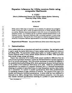
We consider in this section the toy example used to illustrate the Exchange algorithm in (Murray et al., 2006, Section 5). More precisely, the experiment consists of sampling from the posterior distribution of the precision parameter θ arising from the following model: f ( · | θ) = N (0, 1/θ) , p = Gamma(1, 1) , using one observation y =R 2 and pretendingp that the normalizing constant of the 2 likelihood, namely Z(θ) = exp(−θy /2)dy = 2π/θ is intractable. The grid is set as G = {θ˙m = mε, 0 < m ≤ b10/mc}. Our objective is to quantify the bias in distribution generated by the pre-computing algorithms. We consider the situation where the interval between the grid points is ε = 0.1 and n = 10 data are simulated per grid points. Table 1 reports the bias and the variance of the three estimators, i.e. the One Pivot, Direct Path and Full Path, of the ratio Z(θ)/Z(θ0 ) for three couples (θ, θ0 ). This shows that the Full Path estimators enjoys a greater stability than the two other estimators, even when n is relatively small. This is completely in line with the results developed in Propositions 1 and 2. Figure 3 illustrates the convergence of the three pre-computing Markov chains by reporting the estimated total variation distance between π ¯i and π. We also report the convergence of the exchange Markov chain: this serves as a ground truth since π is the stationary distribution of this algorithm. For each algorithm, the total variation distance was estimated by simulating 100, 000 iid copies of the Markov chain of interest and calculating at each iteration the occupation measure. This measure is then compared to π which is, in this example, fully tractable. In view of Table 1, the chains implemented with the One Path and Direct Path estimators converge, as expected, further away from π than the Full Path chain. Interestingly, it can be noted that the Full Path pre-computing chain converges faster than the exchange algorithm. This is an illustration of the observation stated in the introduction regarding the theoretical efficiency of the exchange, compared to that of the plain MH algorithm. Indeed, the pre-computing algorithms aim at approximating MH, and not the exchange algorithm, and should as such inherits MH’s fast rate of convergence, provided that the variance of the estimator is controlled.

17

Pre−computing algorithms, ε=0.1, n=10 exchange One Pivot Direct Path Full Path

0.25

||π−πi||

0.2

0.15

0.1

0.05

0

0

25 i

50

Figure 3: Convergence of the pre-computing Metropolis algorithms distribution. Results were obtained from 100, 000 iid copies of the Markov chains initiated with µ = p. All the chains were implemented with the same proposal kernel, namely θ0 = θ exp σζ, ζ ∼ N (0, 1) and run for 50 iterations. The pre-computing parameters were set to ε = 0.1 and n = 10. Comparing the convergence of the pre-computing chains to that of the exchange (which theoretically converges to π), we see that the Full Path estimator has a negligible bias. This is not the case for the One Pivot and Direct Path implementations.

18

Table 1: Bias and variance of the different estimators of the ratio Z(θ)/Z(θ0 ) for various couples (θ, θ0 ) in the setup of Figure 3. The bias and variance were estimated by simulating 10,000 independent realisations of each estimators for each couple (θ, θ0 ).

FP DP OP

4

(θ, θ0 ) = (1.01, 2.06) bias var. .0007 .005 .003 .208 .004 .199

(θ, θ0 ) = (3.02, 0.55) bias var. .0004 .001 .003 .013 .003 .014

(θ, θ0 ) = (0.12, 0.94) bias var. .01 1.42 .27 99.02 .32 129.81

Results

This section illustrates our algorithm. A simulation study using the Ising model demonstrates the application to a ‘large’ dataset for a single parameter model. More challenging examples are provided with application to a multi-parameter autologistic and Exponential Random Graph Model (ERGM). In the single parameter example we use the estimates of the normalizing constant from Equations (11) and (12), denoted Full Path and Direct Path respectively. For the single parameter example we compare the pre-computing Metropolis algorithm with the standard exchange algorithm (Murray et al., 2006) and also with a version of the methods in Moores et al. (2015). Rather than the Sequential Monte Carlo ABC used in Moores et al. (2015), we implemented their pre-computation approach with a MCMC-ABC algorithm (Majoram et al., 2003). This allowed a fair comparison of expected total variation distance and effective sample size.

MCMC-ABC Moores et al. (2015) used a pre-computing step with Sequential Monte Carlo ABC (see e.g. Del Moral et al. (2006)) to explore the posterior distribution. However, Sequential Monte Carlo has a stopping criterion which results in a finite sample size of values from the posterior distribution. To establish a fair comparison between algorithms whose sample size consistently increases over time, we implemented a modified version of the method proposed in Moores et al. (2015) using the MCMC-ABC algorithm. The modification made to the MCMC-ABC algorithm amounts to replace a draw y 0 ∼ f (·|θ) by a distribution that uses the pre-computed data. More precisely, sufficient statistics of a graph at a particular value θ are sampled from a normal distribution
s ∼ N µ(θ, U), σ 2 (θ, U)} . The parameters µ( · , U) and σ 2 ( · , U) are interpolated using the mean and variance of the pre-computed sufficient statistics obtained at the grid points. This pre-computing version of ABC-MCMC is described in Algorithm 3.

19

Algorithm 3 Pre-computing MCMC-ABC sampler Require: Initial distribution ν, a proposal kernel h and ABC tolerance parameter  > 0 1: Apply the pre-computing step detailed in Moores et al. (2015) pre-computed data U0 . 2: Draw θ0 ∼ ν 3: for i = 1, 2, . . . do 4: Draw θ0 ∼ h( · |θi−1 ) 5: Calculate the mean µ0 and variance σ 02 using the interpolation method in Moores et al. (2015) and the pre-computed data U0 for the parameter θ0 6: Simulate the sufficient statistic s0 ∼ N (µ, σ 02 ) 7: Set θi = θ0 with probability αABC (θ, θ0 , U) := 1 ∧

π(θ0 )h(θi−1 |θ0 ) × 1|s0 −s(y)|