Institute of Computer System, Northeastern University, Shenyang, China ... and queries on parts of XML data require less
Efficient Query Processing for Streamed XML Fragments Huan Huo, Guoren Wang, Xiaoyun Hui, Rui Zhou, Bo Ning, and Chuan Xiao Institute of Computer System, Northeastern University, Shenyang, China
[email protected]
Abstract. Unlike in traditional >315.25 ... ...
...... 2
314
vendor
vendor 4
3
item s
nam e
......
5
W al-M art
item 6
7
93
315
316
nam e
item s
Carrefour ……
......
item 8
9
nam e
m ak e
m odel
pric e
P DA
HP
P alm P ilot
315.25
US D c urrenc y
Fig. 1. An XML Document and its DOM Tree
In [5], a query algebra for XQuery that operates on fragmented XML stream id =" 1" Filler=" tru e" >
Fig. 2. Tag Structure of Hole-Filler Model
Here, we encode the tag attribute “ID” and “Filler” together as a tag code. For “F iller = true”, we set the end of the tag code with “1”, otherwise we set it with “0”. And for attribute “ID”, we separate it from the “Filler” code by a point. The tag code for tag ”vendor” in the previous example is 2.1, while the tag code for tag “items” is 4.0. In this way, we can obtain the fragmentation information by checking the end of the tag code. Figure 3 gives two fragments of the XML document in Figure 1. Here, we number the root filler (i.e. the root of the fragmented document) with f id 0. And other filler IDs can be generated by pre-order traversing XML document tree at the server site. Attribute tsid [4](i.e. tag structure id) indicates the ID of the fragment’s root element in XML document DTD. We associate fillers with holes by matching filler IDs with hole IDs. Fragment 2’s f id corresponds to a Fragment 1’s hid, which means Fragment 2 fills the corresponding hole in Fragment 1 as a subtree when reconstructing the XML document. It is obvious that the contents in Fragment 1 remain relative stable to Fragment 2, i.e. texts (or elements) in Fragment 2 ( such as ”price”) may be updated more frequently. We can save transmission cost by sending Fragment 2 rather than the whole XML document. Furthermore, we can cut ”price” as a single fragment to save update transmission cost. This will lead to higher cost in querying item/price, for the elements now are in two different fragments. There is a trade-off between transmission cost and query cost. In this paper, we assume that XML documents have been fragmented already. What we focus on is query execution on XML streaming fragments at client site. Fragmenting algorithm is stated in [14] and omitted here.
Fragm ent 1: W al-Mart ... ....
Fragm ent 2: PDA HP Palm Pilot 315.25
Fig. 3. XML document Fragments
4
XFPro Query Handling
Based on hole-filler model, infinite XML streams turn out to be a sequence of XML fragments, which become the basic processing units of the query. However, input queries evaluate the elements in the XML document, not the XML fragments. Since fragments with the same tag code share the same structure, we can skip evaluating the structural relationship inside the fragments and expedite processing time by rewriting the queries for XML fragments. This section focuses on the analysis and optimization we perform for queries on fragments. Our goal is to correctly rewrite the query so that it can be processed directly on fragments, and to prune off the redundant path evaluations. Initially, we give an overview of our framework. 4.1
Overview
In this paper, we consider the class of XPath queries that are formed using only the following axes: child, attribute, or descendant axes, denoted as forward XPath. The following query, referred to as Query 1, is an example on the XML document described in Section 1. Query 1: /commodities/vendor/items/item[name=‘‘PDA’’]/price The analysis we perform in this paper is based on the following key observations on queries over streamed XML fragments. In a path expression consisting of predecessor node and successor node, operation dependence (see definition 6)occurs if the following conditions hold true: – The query result to predecessor node and successor node are in the same fragment, or – Any fragment matching the predecessor node also matches the successor nodes. The first condition is straightforward. Let us consider the second condition. When the query nodes involve predicates, the result set of the successor query
must be a subset of that of the predecessor query. When the query nodes have no predicates, the first condition holds true, which means that the query result only depends on the predecessor node. Queries that satisfy this propriety are referred to as subsumption dependence [15], which in most cases can be made subsumption-free by removing the successor nodes. Take Query 1 for example. According to the fragmentation information indicated in tag structure, “commodities”, “vendor” and “item” are root nodes of the fillers while “items”, “price” and“name” are not. Considering that a “vendor” fragment with tsid 5, filler id 7 and hole ids from 10 to 100, arrives and is evaluated against the path expression from query node “commodities”, since query nodes “items” and “vendor” belong to a common fragment according to the fragmentation information in tag structure, fragments that match ”vendor” obviously match “items”(without considering predicates). And such fragments need not to be evaluated for structural relationship between “vendor” and “items”. Much of our analysis bases on such query operation dependencies. Figure 4 shows the key phases in our XFPro system. First, we construct the tid tree from query expression and tag structure. Then, according to tag structure, we apply a series of policies to prune and optimize the tid tree. Such techniques not only rewrite some queries to avoid redundant operations, but most importantly, they save the memory space and processing power. After optimization, we transform the tid tree into query processor, and efficient query execution plan is generated. XFPro Framework Query Transformer
Query Plan Generator
Path Expressions
Optimized Tid Tree
Tid Tree
XFPro Query Engine
Prune Policy
Query Plan
Fig. 4. Overview of the Framework
4.2
Tid Tree
We introduce tid tree to represent the query expression and enable further analysis and optimizations on query operations. Definition 5. Let N be the set of query nodes in a query Q. Tid tree is a tree T T = (Tt , Et , roott , Pt , Ot ), where Tt is the set of corresponding tag codes of the nodes in set N; Et is a set of edges describing the structural relationship between two nodes; Pt is a text set of the predicate values; Ot is an operator set including boolean connectors; roott (∈ Vt ) is the root element of the tree.
We introduce subroot node denoted as the root of a filler, and subelement node that locates in a filler but is not the root of the subtree. By taking advantage of tag codes, we can easily tell subroot nodes from subelement nodes by checking the end of the code. And parent-child relationship between nodes is represented by a single arrow, while ancestor-descendant relationship between nodes is represented by a double arrow. In the case that the descendant node corresponds to multiple tag codes, we duplicate the descendant node and assign different tag codes to them (see Section 4.3 for details). The output of the query is depicted by an arrow. In order to distinguish between the node that represents a tag code and the node that represents an atomic predicate, we represent tag nodes with circles and values of predicates with rectangles. The operators (such as , ≥, ≤, =) and boolean connectors are represented with diamonds. The tid tree for the Query 1 described in the previous section is shown in Figure 5. 1.1 is the tag code of “commodities” and similarly, 2.1, 4.0, 5.1, 6.0 and 7.0 are the tag codes of “vendor”, “items”, “item”, “price” and “name”. Here, “=” and “PDA” are treated as operator node and predicate node respectively in the tid tree.
1.1
2.1
4.0
5.1
7.0
= 6.0
"PDA"
Fig. 5. Tid Tree of Query 1
4.3
Optimizing Tid Tree
In XFrag [4], each query primitive corresponds to an XFrag operator, which processes the fragment only if the tsid of the fragment matches that of the operator. In the case that they do not match, the fragment is simply passed on to the subsequent operator in the query tree. However, in the case of operator dependence (as illustrated in Section 4.1), the fragments that do not match the predecessor operator need not to be evaluated against the successive one. Definition 6. Given any pair of nodes in tid tree n1 ,n2 , if the query result of n2 is valid only if that of n1 is valid, n2 is considered dependent on n1 . We use directed edge e = (n1 , n2 ) to imply the dependence between n1 and n2 . Definition 7. Given any pair of nodes in tid tree n1 ,n2 , n2 is subsumption dependent on n1 if: (i) n2 is dependent on n1 , and (ii) the query result of n2 is a subset of the query result of n1 . Subsumption-free queries are intuitively queries that do not contain “redundancies”. Some queries can be rewritten to be subsumption-free, by eliminating
redundant portions. Much of our analysis focuses on finding such dependencies on tsid nodes, to eliminate “redundant” query evaluations on structural relationship. In pruning process, we use dashed arrows to represent subsumption dependencies, and solid arrows for subsumption-free dependencies. Path Pattern Query Path pattern query is the simplest type of queries. Meanwhile it is the base of tree pattern query. Firstly, we assume that the query does not contain “//” and “*”. This class of query covers most of the structural relationship “redundancies”. For example, Query 2 is a simple path pattern query with only “/” involved. Query 2: /commodities/vendor/items/item/name The original query involves three fragments with tsid 1, tsid 2 and tsid 5 and the tid tree includes five steps with tsid 1, tsid 2, tsid 4, tsid 5 and tsid 6. However, since fragments that don’t match tsid 2 obviously don’t match tsid 4, i.e. tsid 4 subsumption depends on tsid 2. We can rewrite the query to avoid such redundant operations by deleting subelement nodes which have no predicates and are not the leaf nodes in tid tree. According to tag code, subroot nodes ended with “1” are kept in the tid tree while subelement nodes ended with “0” and without predicate node in their children are removed. Since tsid 6 is a subelement node with predicate and tsid 7 is the leaf node in tid tree, they are kept in the tree. Figure 6 shows the optimized tid tree after pruning off the dependent node 4.0 (depicted by “X”).
1.1
2.1
4.0
5.1
6.0
Fig. 6. The Pruned Tid Tree after removing Subsumption Dependence of Query 2
However, pruning path pattern query may lead to incorrect results, when “//” and “*” are considered. This is because the ancestor node A before “//” and the descendant node D after “//” may belong to different fragments. Hence the fragment matches A may not match D. Similarly, “*” may not match in the same filler and we cannot determine subsumption dependence directly. In such cases, we need to rewrite the tid tree into “//” or “*” excluded form. Taking “//” for consideration, we first capture all the paths from A to D when traversing the tag structure. Then we insert the tag codes of corresponding subroot nodes of D into tid tree and link them with A according to the path. In this way, “//” is replaced by “/” and the query result is the merge set of each output node in tid tree. Now we can apply the pruning scheme for “/” to the rewritten tid tree. Figure 7 presents the tid tree of Query 3, which returns the descendants “name” of “vendor”.
4.4
Query Plan Generation
As described in the previous section, we rewrite original query into tid tree. However, the tid tree only represents a view of relationships between tsid nodes and predicates, while the details of query processing are not modelled. This section focuses on the transformation from tid tree to the corresponding query plan and gives a processing example of XFPro.
1.1
1.1
2.1
2.1 "PDA" 5.1
= 6.0
5.1 result
=
7.0
HAS H T ABLE
7.0
6.0
''PD A ''
BUC KET
Fig. 9. Transformation from Tid Tree to XFPro
The transformation from tid tree of Query 1 into the XFPro processor is depicted in Figure 9. Each subroot node in tid tree corresponds to an entry of hash table, which is tagged by a value of true, false, undecided (⊥). And each subelement node is added in a bucket tagged by an odd value linked to the corresponding entry of the subroot node, while each predicate node is added in a bucket tagged by an even value linked to the corresponding entry. There is a result entry at the end of the hash table, which has a linked bucket to cache the candidate output. It conjuncts all the entries’ value and is set true only if all the predecessor entries are set true. The XFPro processing for Query 1 is depicted in Figure 10. When the “commodities” fragment with tsid “1”, filler id “0” and hole ids “1, 21, 41” arrives, the query hash table set the entry 1 with T and the information is saved in the bucket linked to the entry. More over, the fragment with tsid “1” is tagged with an undecided value when it has predicate and the condition has not been evaluated for this fragment. Note that, at the point, the “commodities” filler can be discarded as it is no more needed to produce the result and the hole filler association is already captured. This results in memory conservation on the fly. Similarly, when the “vendor” fragment with the corresponding tsid “2” arrives, the entry 2 saves the information into the bucket and is set T , as there is no condition for it. When the “item” fragment with tsid “5”, filler id “3” arrives, the entry 5 is set ‘⊥’, since it has predicate bucket. After determining that the information in filler “3” matches the predicate, it sets the entry T . The “item” fragment may also be discarded at the point conserving memory, for the result value, which is a subset of the fragment, is already captured in the linked bucket. Since all the entries in the hash table are set “true”, the value of price is output as the result. The algorithms listed below describe the processing method.
T tsid= 1 fid= 0 hid (1, 21,41)
tsid= 1 fid= 0 hid (1,21,41)
2.1 5.1
6.0
7.0
result
T T tsid= 5 fid= 3
tsid= 2 fid= 1 hid (2,...,20)
5.1
7.0
6.0
=
tsid= 1 fid= 0 hid (1,21,41) tsid= 2 fid= 1 hid (2,...,20)
T
tsid= 1 fid= 0
T
tsid= 2 fid= 1 hid (2,...,20)
T
315.25
T =
BUCKET
''P D A ' '
HASH TABLE BUCKET (2 )
result
HASH TABLE (3 )
T
''P D A ' '
BUCKET
name
hid (--)
tsid= 1 fid= 0 hid (1,21,41)
result =
HASH TABLE (1 )
tsid= 2 fid= 1 hid (2,3,...,20)
T
hid (1,21,41)
T
315.25
315.25
''P D A ' '
=
''P D A ' '
HASH TABLE BUCKET (4 )
Fig. 10. XFPro Processing Example
Algorithm1 FindQueryChild() {Input an element node and trigger descendant operators} IF (isHashTerminalNode(element)) THEN output element; ELSE q