Efficient Rendering of Atmospheric Phenomena - Purdue Engineering

Eurographics Symposium on Rendering (2004) H. W. Jensen, A. Keller (Editors)

Efficient Rendering of Atmospheric Phenomena Kirk Riley† , David S. Ebert† , Martin Kraus† , Jerry Tessendorf‡ , and Charles Hansen§

Abstract Rendering of atmospheric bodies involves modeling the complex interaction of light throughout the highly scattering medium of water and air particles. Scattering by these particles creates many well-known atmospheric optical phenomena including rainbows, halos, the corona, and the glory. Unfortunately, most radiative transport approximations in computer graphics are ill-suited to render complex angularly dependent effects in the presence of multiple scattering at reasonable frame rates. Therefore, this paper introduces a multiple-model lighting system that efficiently captures these essential atmospheric effects. We have solved the rendering of fine angularly dependent effects in the presence of multiple scattering by designing a lighting approximation based upon multiple scattering phase functions. This model captures gradual blurring of chromatic atmospheric optical phenomena by handling the gradual angular spreading of the sunlight as it experiences multiple scattering events with anisotropic scattering particles. It has been designed to take advantage of modern graphics hardware; thus, it is capable of rendering these effects at near interactive frame rates. Categories and Subject Descriptors (according to ACM CCS): I.3.7 [Computer Graphics]: Three-Dimensional Graphics and Realism Color, shading, shadowing, and texture

1. Introduction Particles in the atmosphere are responsible for a wide range of optical phenomena. Wavelength-dependent effects, such as the arcs of rainbows, cirrus halos, and the glory, are just a few [Min93]. These effects add beauty and realism to outdoor scenes; thus, the capability to render these effects accurately is an important component of an outdoor renderer. Unfortunately, physically accurate radiative transfer is a notoriously difficult problem because the number of possible paths photons may take through a cloud volume grows exponentially with the expected number of scattering events. Multiple scattering in a highly scattering medium, such as a cloud, has long been recognized [KVH84] as an essential lighting component. Multiple scattering blurs source light both angularly and spatially. Thus, the process of multiple scattering gradually blurs out fine angularly dependent effects from the phase function, as the light distribution becomes more isotropic traversing the cloud. Modeling the angular distribution of light as it interacts with anisotropic scat† Purdue University ‡ Rhythm and Hues § University of Utah c The Eurographics Association 2004.

tering particles is a difficult problem and, therefore, it is often over-simplified, or even ignored, in most graphics applications. An accurate lighting model in clouds must produce both single-scattering effects, as well as diffusive illumination. Unfortunately, lighting models either cannot handle both, or require an arbitrarily long time to do so. We have solved this problem through the use of multiple scattering phase functions to model the gradual loss of angular coherence in the light beam. Our algorithm takes full advantage of the power and flexibility offered by modern programmable graphics hardware. Therefore, this system efficiently renders single and multiple scattering atmospheric effects with aerial perspective, while maintaining reasonable rendering times. In Section 2, we provide the background for rendering atmospheric data and skylight. In Section 3, we describe the atmospheric particle data we are rendering. Next, in Section 4, we discuss the rendering and lighting model used in our system. Some implementation details are given in Section 5. Then, in Section 6, we present our results. Finally, conclusions and future work are given in Section 7 and Section 8 respectively.

K.Riley, D. Ebert, M. Kraus, J. Tessendorf & C. Hansen / Efficient Rendering of Atmospheric Phenomena

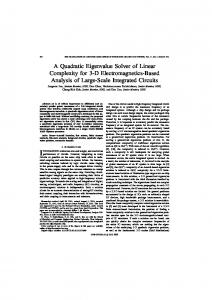
Figure 1: Cirrus sunrise time sequence

2. Previous Work Rendering of outdoor and highly diffusive media has been an active area in computer graphics for more than ten years. The single-scattering low-albedo model [Bli82] provides the framework for rendering particle fields. Early work in modeling multiple scattering involved spherical harmonics [KVH84] and volumetric radiosity solutions [RT87]. More recent diffusion systems model light with a first order angular distribution using a multi-grid scheme [Sta95], with multiple order scattering reference patterns [NDN96], and with multiple anisotropic scattering [MSM∗ 04]. The subsurface light transport system [JMLH01] calculates a diffusion approximation by applying the dipole method to meet boundary conditions at the surface. This method is well suited for reasonably flat boundaries between two homogeneous regions but is less suited for a volumetrically varying inhomogeneous volume, such as multiple-particle clouds. Additionally, diffusion approximations tend to blur fine angularly dependent effects quickly, and are less suited to rendering fine angularly dependent effects in volumes, than the technique presented here. This is particularly evident in the case of larger particles, where, for unity albedo, it may take more than 25 scattering events before the distribution is essentially isotropic. Discrete ordinates [Max94], photon mapping [JC98], and path integral methods [PAS03, Tes87] can generate high accuracy solutions but are computationally expensive when fine angularly dependent effects are desired. Volume rendering [DCH88] has been widely applied in computer graphics and has been extended to gaseous volume rendering [SF95, EP90, REHL03]. Hardware-accelerated techniques in atmospheric modeling and rendering include imposter systems [HL01], cloud formation modeling systems [HBSL03], and intuitive modeling systems [SSEH03]. The small angle approximation [KPH∗ 03, KPHE02], which has been applied to atmospheric rendering [REHL03], is efficient but discards the phase effects after the first scattering event. These hardwareaccelerated systems have increased the efficiency of atmospheric rendering systems but have not achieved the capability to render fine angularly dependent effects. Advanced phase function effects are an essential component of an atmospheric renderer. Rendering rainbows with Descartes’ ray tracing method [Mus89] for rain drop phase function calculation has been presented. Complex phase functions and rendering advanced atmospheric optical ef-

fects have been achieved for a single-scattering lighting model [JW97]. Halos and parhelia have also been discussed for ray-tracing [JW98]. While advanced phase functions have been considered in computer graphics, they have not been used in an interactive system that models the gradual angular spreading of the source light. These atmospheric rendering options, while useful, make significant simplifications to the light’s angular distribution, the phase function, or both. A common approximation is to estimate scattering phase based on a function of the first moment of the phase function and the dot product of the incident and exit directions [Bli82, SF95, MSM∗ 04, Sta95, NSTN93], such as the Henyey-Greenstein function. This results in an oversimplification of the angular distribution of the light that eliminates fine angular dependent effects. Here, we present a system that is capable of modeling both a complex lighting distribution and a complex phase function that can capture the effects of both the angular spreading and diffusion of light, and the optical effects of advanced phase functions. Rendering the sky is another essential element of rendering outdoor scenes. The two density layer scheme [Kla87] provided the ground work for rendering the sky. The basis function method [NSTN93] is very efficient but is less suited for the addition of interacting media. An efficient physicallybased sky light approximation [PSS99] has been presented for ground observers. A physically accurate system for modeling the skylight at night has also been described [JDS∗ 01]. Numerical integration techniques [EMP∗ 03] also provide accurate solutions to generating aerial perspective and skylight. While these schemes are very useful, we propose a hardware-accelerated method of rendering the sky that allows us to use an analytical expression and, thus, achieve a sky that interacts with the atmospheric data at reasonable rendering speeds. 3. Atmospheric Data The atmosphere is an inhomogeneous mixture of a wide variety of particles. In order to develop a system for the accurate rendering of these particles, it is essential to first specify the particles’ properties as described in Section 3.1. We then translate these properties into the spatially varying scattering probabilities and phase functions required to volumetrically render the particle fields in Section 3.2. c The Eurographics Association 2004.

K.Riley, D. Ebert, M. Kraus, J. Tessendorf & C. Hansen / Efficient Rendering of Atmospheric Phenomena

Variable λ

Figure 2: Rain Mie phase function for red, green, and blue wavelengths

3.1. Particle Properties We assume atmospheric bodies primarily consist of two types of high-albedo particles and that dirt and other particle types have a minimal contribution. We also assume that the renderer will only consider wavelengths in the visible spectrum (between 400 and 700 nm), where these particle properties are accurate.

α Amsλn Aλ (~s 0 , Ω) βλex βsca ∆ I λ (~s 0 ) λ Lλ (~s, Ω) ~mΩ n(~s) Ω Ω−Ω0 Ωlt ~pΩ Pλ (Ω) λ P (Ω − Ω 0 ,~s 0 ) ~s ~sbg (~s, Ω) σλex λ T (~s,~s 0 ) ξ

Definition single-scattering albedo (βλsca /βλex ) multiple scattering angular distribution angular distribution function extinction coefficient (m−1 ) scattering coefficient (m−1 ) slice spacing (m) total intensity for all directions at ~s 0 light wavelength (nm) light intensity normalized vector in Ω direction expected number of scattering events direction scalar angle between directions (radians) sunlight direction opposite Ω normalized vector particle single-scattering phase function combined (spatial) phase function 3-D point in space background point for this ray extinction cross-section (m2 ) transparency between ~s and ~s 0 User adjustable back-scattering contribution

Table 1: Variable and parameter descriptions

The first particle type we consider consists of air molecules characterized by highly wavelength-dependent scattering probabilities, yet comparatively isotropic Rayleigh scattering and a wavelength-independent phase function. The second type consists of larger ice and water particles with nearly wavelength-independent scattering probabilities and strongly forward peaked wavelengthdependent phase functions. Specifically, the water particles we consider are classified as cloud (small spherical water), rain (large spherical water), ice (hexagonal ice cylinders) and snow (random ice crystals), but the system does not currently render haze, fog, or more complex ice particles such as graupel. Because scattering behavior is vastly different between the two types of particles, we use different lighting models for each. The scattering from atmospheric particles are characterized by wavelength-dependent parameters including extinction cross-section (σλex ), the single-scattering albedo (αλ ), and the single-scattering phase function (Pλ (Ω)), summarized in Table 1.

unity albedo, atmospheric particles have near unity albedos in visible wavelengths [KYBN02, CS92]; therefore, we assume all the particle albedos are one.

As described before, the extinction cross-section is highly wavelength-dependent for air particles and not wavelengthdependent for the larger particles. Therefore, σλex = σex for water particles. For large spherical particles, the extinction cross-section is approximately twice the geometric crosssection, σex = 2πr2 [LLO∗ 91]. The scattering cross-section is σsca = ασex , where α is the single-scattering albedo. The extinction cross-sections of the particles used in our system are given in Table 2. Although the system is not limited to

The scattering phase function for these particles, Pλ (Ω), is the probability density function describing the angular deflection of light (Ω) after an interaction with the particle. In general, Ω is a vector, but for randomly oriented particles, Pλ (Ω) is a function of the scalar angle between the incoming and outgoing (after scattering) directions. This assumption, valid for a turbulent atmosphere, eliminates some ice crystal optical phenomena, such as parhelia, but simplifies the model substantially. The Rayleigh phase function for air

c The Eurographics Association 2004.

Attribute

σex (m2 )

Air at 650 nm Air at 515 nm Air at 440 nm Cloud (0.01 mm sphere) Rain (1 mm sphere) Ice Snow

2.28 × 10−31 5.33 × 10−31 1.30 × 10−30 6.28 × 10−10 6.28 × 10−6 1.82 × 10−6 1.41 × 10−5

Table 2: Atmospheric particle extinction cross-sections

K.Riley, D. Ebert, M. Kraus, J. Tessendorf & C. Hansen / Efficient Rendering of Atmospheric Phenomena

For ice, we assume random orientation such that the phase function is dependent solely on the angle between the eye and light rays. The phase data is taken from Hess and Wiegner’s Cirrus Optical Properties system [HW94]. A plot of the ice phase function for green light is also shown in Figure 3. The peaks of this ice phase function at 22 and 46 degrees create halos of color when the sun penetrates optically thin cirrus clouds, such as in Figure 6. The other wavelengths have skewed values at the peaks at 22 and 46 degrees, making these halos chromatic phenomena. 3.2. Rendering Properties Figure 3: Phase of all particle fields for green light

One quantity of interest for calculating light transport is the extinction coefficient, βex . This is the probability, per meter, that light intersects a particle. As described by Blinn [Bli82], this can be calculated by multiplying the particle density with the extinction cross-section. At a point in space, ~s, this is calculated as the following: βex (~s) = η(~s)σex .

(2)

Here η is the particle concentration in particles per cubic meter. For multiple particle fields, the extinction coefficients linearly combine.

∑

βex (~s) =

(i)

all fields i

Figure 4: Glory in cumulus cloud

(3)

The optical depth, τ, along a segment between ~s and~s 0 is the integral of the extinction coefficient along the ray. τ(~s,~s 0 ) =

molecules is given in Equation 1.  3  Pair (Ω) = 1 + cos2 (Ω) (1) 16π Mie scattering dominates for homogeneous spheres much larger than the wavelength of light, and describes rain and cloud particle phase functions. We use Philip Laven’s MiePlot [Lav], an implementation of Bohren and Huffman’s [BH83] Mie code, to calculate the Mie phase function at an angular resolution of 0.1 degrees. Additionally, because rain and clouds are actually a collection of randomly distributed particles, we calculate the phase function using a lognormal distribution for the particle size, with parameters described by Pruppacher and Klett [PK00]. The rain phase function is given in Figure 2. For comparison, Figure 3 is a plot of the phase functions for green light for all particle fields. Cloud water has a similar behavior, with a milder forward peak and more relaxed peaks at rainbow angles as shown in Figure 3. Wavelength dependence for the peaks near 180 degrees in the cloud water phase functions create the glory: tight rings of color reflected backward towards the sun, as shown in Figure 4. Notice the double peaks around 120 and 140 degrees for rain. The wavelength dependence of these peaks causes rainbows, like the one in Figure 5; the lull between them is Alexander’s dark band.

βex (~s)

Z ~s 0 ~s

βex (~s 00 )ds00

(4)

The transparency, T , of the medium is then: T (~s,~s 0 ) = e−τ(~s,~s ) . 0

(5)

The total phase function at a point in space is calculated by weighting each of the individual particle phase functions by their contribution to the total scattering coefficient.

∑

P(Ω,~s) =

(i)

all fields i

α(i) βex (~s)P(i) (Ω)

∑

(i)

all fields i

α(i) βex (~s)

(6)

Now that we have a system for calculating the spatially varying properties of the particle fields, we shift our attention to a system for rendering these particles that can capture realistic illumination effects. 4. Rendering Atmospheric Data Our efficient rendering of atmospheric data is accomplished by combining several rendering models. The first is a singlescattering sky-rendering approximation. Single-scattering is used because, for altitude angles greater than about 16 degrees, and with a flat earth, the expected number of air scattering events along a view ray is less than one. This angle c The Eurographics Association 2004.

K.Riley, D. Ebert, M. Kraus, J. Tessendorf & C. Hansen / Efficient Rendering of Atmospheric Phenomena

Figure 5: Rainbow in rain field of a storm

Figure 7: Rendering system flow diagram (front-to-back)

Figure 6: Halo in a cirrus cloud

is even smaller for a round earth, as the height will increase faster with distance. Calculation of the sky attenuation and sky lighting terms are given in Section 4.1. For rendering the larger water and ice particles, we utilize a model based upon multiple scattering phase functions described in Section 4.2. At its core, this is a volume rendering application that renders multi-field atmospheric data on a uniform voxel grid, containing particle density (η(~s)) values. It applies the half angle slicing scheme for a light buffer and an eye buffer, as presented in Kniss et al. [KPH∗ 03]. This method slices volume data at an angle suitable for both the eye and light perspectives, i.e. at the angle halfway between them. Rendering is done both to an eye (or image) buffer to accumulate light directed into the eye rays, and to a light buffer, which stores the attenuation of light as it traverses the volume. A diagram showing the flow of the full system is given in Figure 7. For front to back rendering, a slice halfway through the volume that covers the entire image is rendered first, to estimate atmospheric inscattering between the eye and the volume. Then, half-angle slicing is performed on the volume, alternating between compositing in the eye buffer, and attenuating in the light buffer. c The Eurographics Association 2004.

Figure 8: Rendering system overview

Finally, the atmosphere behind the cloud is approximated by calculating all atmospheric inscattering from the plane halfway through the volume onward, and this result is composited into the image. To get an overview of which system components render which model components, an overview image is given in Figure 8. A general light transport equation, relating the light intensity at ~s in the direction Ω to the light intensity everywhere

K.Riley, D. Ebert, M. Kraus, J. Tessendorf & C. Hansen / Efficient Rendering of Atmospheric Phenomena

else, is given in Equation 7 [Cha60]. λ

λ

λ

L (~s, Ω) = L (~sbg (~s, Ω), Ω)T (~sbg (~s, Ω),~s) + Z ~s

~sbg (~s,Ω)

Z

4π

T λ (~s,~s 0 )βλsca (~s 0 ) ×

Pλ (Ω − Ω 0 ,~s 0 )Lλ (~s 0 , Ω 0 )dΩ 0 ds0

(7)

Note that~sbg (~s, Ω) is the background point found by traversing from ~s in the direction opposite Ω until it intersects with the background, which may be the sun, the earth, or space. Also note that Ω − Ω 0 represents the scalar angle between the direction vectors Ω and Ω 0 . Equation 7 says that the light at ~s in the direction Ω equals the background intensity defined by ~s and Ω times the transparency through the volume, plus the contribution from inscattering at all points along the ray. The difficult issue is that the light distribution at all points along the ray must be known to calculate the light intensity in a single direction reaching a point along that ray. We now present an analytic aerial perspective model that simplifies this equation with a single-scattering approximation. 4.1. Aerial Perspective Both aerial perspective and skylight are essential in an atmospheric renderer. Aerial perspective (the blueing of distant dark objects during the day, and the reddening of bright objects at dusk and dawn) is an essential outdoor depth cue, while proper skylight is required for any realistic outdoor scene renderer. It is often desirable to render atmospheric bodies from any perspective and, therefore, we do not limit the observer to be on the ground. Direct sunlight is accounted for separately, in Section 4.2.4. Therefore, the single-scattering analytic model presented here has zero background intensity. We also assume sunlight to be collimated; thus, we need only consider the direction of the sun, Ωlt , in the directional integral over Ω. Air consists of a consistent mixture of molecules, and, therefore, the phase function of the particles does not change with spatial location. Hence, for atmospheric inscattering, Equation 7 quickly reduces to something more manageable in Equation 8. Lλ (~s, Ω) =

Z ~s

~sbg (~s,Ω)

T λ (~s,~s 0 )βλsca (~s 0 ) ×

Pair (Ω − Ωlt )Lλ (~s 0 , Ωlt )ds0

(8)

It is clear that Pair does not depend on the point in space, and is factored. Therefore, we need only concern ourselves with the three other terms. We first calculate the scattering coefficient. We then consider how to find the transparency from the sample to the eye. Next, we calculate the light value at the sample, assuming the sun is at infinity. Finally, we put it all together into an analytic expression for the light directed toward the eye.

Wavelength (nm)

βsl

680 550 440

5.8 × 10−6 m−1 1.35 × 10−5 m−1 3.31 × 10−5 m−1

Table 3: Sea-level scattering coefficients

4.1.1. Scattering Coefficient Like Nishita et al. [NSTN93] and Preetham et al. [PSS99], we make the hydrostatic approximation that the atmosphere has an exponentially decreasing particle density from sealevel as shown in Equation 9. η(h) = 2.55 × 1025 e−γh m−3

(9)

The scattering coefficient is then the scattering cross-section times this particle density. We use a single-scattering model to calculate the aerial perspective because of its analytic simplicity and because we expect few scattering events as sunlight traverses the atmosphere. Since the scattering coefficient is linear in particle concentration, η, the scattering coefficient is an exponentially decreasing function of height. βλsca (h) = βλsl e−γh

(10)

h is the height above sea-level. In this model, the lapse rate 1 is γ = 8000 m . The βsl values we use for the three color channels (red, green, and blue) are given in Table 3. Now that we have an expression for the scattering coefficient, we can calculate the transparency of the atmosphere. 4.1.2. Atmospheric Transparency Air molecules have high albedo and, thus, the probability of extinction (any mechanism for removing light from a ray) is equal to the probability of scattering, βex = βsca . We assume that the earth is flat, so that the height varies linearly along the ray between two points. Let ~pΩ be the vector in the opposite direction of Ω. Substituting Equation 10 into Equation 5 and performing the integral, we get a solution in terms of the y-component of ~pΩ , pΩy , the scattering coefficient at sea-level, βλsl , the height of ~s, sy , the distance between ~s and ~s 0 , denoted K, and the lapse rate, γ. !  βλsl −γsy  −γpΩy K λ 0 T (~s,~s ) = exp − (11) 1−e e γpΩy Thus, we have an expression for the transparency of the atmosphere between two points. We use this to calculate the atmospheric attenuation of light to a point, and to find the attenuation from that point to the eye. 4.1.3. Sample Lighting The last component needed to solve the overall light transport equation is the light value at a point in space, L(~s, Ωlt ). If c The Eurographics Association 2004.

K.Riley, D. Ebert, M. Kraus, J. Tessendorf & C. Hansen / Efficient Rendering of Atmospheric Phenomena

Lλ (~s, Ω) = Pair (Ω − Ωlt ) × ! Z ~s  βλ   exp − eye 1 − e−γpΩy K × γpΩy ~sbg (~s,Ω) ! βλsl −γs0y  0 λ −γs0y λ Is exp − e βsl e ds γly 

(14)

Now, recognizing that s0y = pΩy K +sy , we solve this integral, and get a final expression in Equation 15 for the skylight reaching the eye from all points along a ray between ~s and a sample that is K away, ~s 0 .

Figure 9: Sky and aerial perspective

ly × pΩy − ly       exp − 1 βλeye 1 − 1 e−γpΩy K − γ ly pΩy     1 1 λ 1  exp − βeye − γ ly pΩy Lλ (~s, Ω) = Isλ Pair (Ω − Ωlt )

Figure 10: Uniform background sky, no aerial perspective

we set the sun intensity outside the atmosphere to be Isλ , then we simply use Equation 11 to attenuate this intensity. Let l be the normalized vector pointing towards the sun. Therefore, we are only interested in the initial height of the sample, s0y , and the y-component of l, ly . If we assume that ly is positive for a daylight scene (the light must always be above the horizon) and let the distance go to infinity, the integral converges to Equation 12.   0 β (12) Lλ (~s 0 , Ωlt ) = Isλ exp − sl e−γsy γly We now have an expression for all quantities in Equation 8 and can calculate the amount of inscattering along the eye ray between two points. 4.1.4. Analytic Sky Model Finally, we derive an expression for the amount of atmospheric inscattering of light into a ray along a given distance. To simplify, let βeye be the scattering coefficient at the eye. βλeye = βλsl e−γsy

(13)

If we substitute Equations 10, 11, and 12 into Equation 8 we get an equation of the form:

(15)

This approximation produces realistic sky results, as shown in Figure 9. For comparison, the same cloud without the sky and aerial perspective is shown in Figure 10. Note that the hue in darker regions of this very large cloud model are more blue in the rendering with aerial perspective than the rendering without. Additionally, this skylight and atmospheric attenuation creates the characteristic reddening of objects at sunrise and sunset. This effect can be seen in the dawn images of cumulus clouds, in Figures 1 and 11, and a cirrus in Figure 12. Now that we have a model for the sky attenuation and source, we present our approximation for multiple scattering in the light volume. 4.2. Multiple Scattering Phase Function Lighting Approximation We have developed a model for the angular dispersion of light as it experiences its first few scattering events traversing the volume. This model has been designed for efficient rendering in a single pass through the volume, taking advantage of programmable graphics hardware. This technique extends the half-angle slicing technique described by Kniss et al. [KPHE02] to handle the gradual angular spreading of light as it undergoes multiple scattering, rather than only considering unscattered and diffuse light. This is essential for capturing fine angularly dependent effects in the presence of large atmospheric scattering particles, which highly favor forward scattering. As mentioned previously, the difficulty with Equation 7 is the presence of Lλ on both sides of the equation. To approximate this equation, we first separate Lλ (~s, Ω) into its

c The Eurographics Association 2004.

K.Riley, D. Ebert, M. Kraus, J. Tessendorf & C. Hansen / Efficient Rendering of Atmospheric Phenomena

4.2.1. Estimating Angular Distribution Since we have separated the light contribution into intensity and distribution, we utilize Equation 18 and rewrite Equation 7 into the form in Equation 19. I λ (~s)Aλ (~s, Ω) = Isλ δ(Ω − Ωlt )T λ (~sbg (~s, Ω),~s) + {z } | Lλ (~s,Ω)

Z ~s

~sbg (~s,Ω)

Z

4π

I λ (~s 0 )T λ (~s,~s 0 )βλsca (~s 0 ) ×

Pλ (Ω − Ω 0 ,~s 0 )Aλ (~s 0 , Ω 0 )dΩ 0 ds0

(19)

Clearly, the last integral is a spherical convolution in Ω. After a single scattering event, we expect the scattered light to have the angular distribution of the particle phase function. If the light experiences two scattering events, we expect the twice-scattered light to have an angular distribution of the phase function convolved with itself. Therefore, we define a multiple-scattering angular distribution function, Amsλn , to approximate the distribution of light after n scattering events with Equation 20.   λ λ Amsλn (Ω) = δ(Ω − Ωlt ) ∗ P ∗ . . . ∗ P (20) | {z } (Ω)

Figure 11: Cumulus cloud at dawn

n−times

If we assume that, for a small number of scattering events, the angular distribution of Lλ remains peaked in the initial light direction with gradual angular spreading, then we can approximate the angular distribution with this multiple scattering angular distribution function. The expected number of scattering events for a ray is given in Equation 21.

Figure 12: Cirrus cloud with halo at dawn

n(~s) = λ

λ

intensity, I (~s), and its angular distribution, A (~s, Ω). Lλ (~s, Ω) = I λ (~s)Aλ (~s, Ω)

(16)

Aλ , as an angular distribution, is subject to the constraint: Z

4π

Aλ (~s, Ω)dΩ = 1, ∀~s, λ

(17)

The distribution of light, Aλ , is closely tied to the number of scattering events it experiences between the source and the given point in the volume. We make the assumption of a purely collimated initial light source that is then redirected through scattering. Lλ (~sbg (~s, Ω), Ω) = Isλ δ(Ω − Ωlt )

(18)

Therefore, all background intensities are equal and have a single direction. In Section 4.2.1, we describe a method for estimating the angular distribution of the light in the volume. Then, in Section 4.2.2, we develop a system for calculating the intensity of light in the volume using this angular distribution.

Z ~s

~sbg (~s,Ωlt )

γ

αγ βex (~s 0 )ds0

In terms of transparency from the light source:
n(~s) = −α ln T (~s,~sbg (~s, Ωlt )) .

(21)

(22)

We estimate the number of scattering events to be this average number. Note that this is, nominally, a function of the direction and the data along all possible paths, but, for efficiency, we estimate the number of scattering events as this mean. The result is that, by tracking only the transparency of the material traversed from the light source, we can get an approximate expression for the angular distribution of the total intensity at that point. Our system records a single intensity value in a light buffer (see Section 5) and sums the contribution from the previous slice that is directed to the current sample. A preset number of angular distribution functions, Amsλn (Ω), is pre-computed and saved in a floatingpoint precision texture. These functions are calculated for up to n = 26, when the angular distribution function for rain (the worst case with the highest forward peak) becomes isotropic (to within .0001%). c The Eurographics Association 2004.

K.Riley, D. Ebert, M. Kraus, J. Tessendorf & C. Hansen / Efficient Rendering of Atmospheric Phenomena

4.2.2. Intensity Calculation With this approximation for the angular distribution of the light, it is easier to calculate its intensity distribution. This intensity distribution is the quantity stored in the light buffer, and represents the total light intensity reaching the samples. This value, along with its angular distribution is then used to calculate the final gather to the eye, as described in Section 4.2.3. The intensity received at a given sample normally has two components: the unscattered light intensity already directed towards the sample, and the scattered light that has been re-directed into the sample. Because we calculate the scattered angular distribution of light, these are not handled separately. To model the attenuation of light, from one sampling slice to the next, we discard all backward directed light (relative to the direction of the sun) for each scattering event. This is done for two primary reasons. The first is that the phase functions have only a weak back-scattered component. The second is that this system performs a single slicing pass through the volume and, therefore, has no knowledge of the data on future slices. Note that this is for intensity transport in the light buffer only, and that light may still be backscattered towards the eye in the final gather, described in Section 4.2.3. Therefore, we let Fiλ be the forward-scattered contribution after i scatters, i.e., the integral over the forward hemisphere of Amsλi (Ω). Fiλ =

Z

forward hemisphere

Amsλi (Ω)dΩ

(23)

Let ~mΩlt be the vector in the direction of Ω. To get the intensity for the current slice (I(~s + ~mΩlt ∆)), from the intensity on the previous slice (I(~s)), for a discrete number of scattering events, the light is attenuated according to Equation 24. I(~s + ~mΩlt ∆) = I(~s)T (~s,~s + ~mΩlt ∆) + I(~s)(1 − T (~s,~s + ~mΩlt ∆))

n(~s)+dβλex ∆e

∏

i=n(~s)+1

α(~s)Fiλ

optical effects, and is least accurate in dense inner regions of the cloud. 4.2.3. Rendering with Angular Distribution To apply this result, we do a single slicing pass through the volume, collecting the inscattered intensity from the volume samples into the eye ray. For light scattered to the eye, we apply the angular distribution function for one more scattering event than the expected number of scattering events reaching this sample, n(~s f + i~mΩ ∆) + 1, as this scattering event is the one that directs light into the eye ray. Rendering without any backscattered light darkens the region of the cloud where light first strikes it; therefore, a user adjustable term is added to the phase function, ξ. This term models the amount of light the system will receive back from multiple scattering further along the path. If we assume front-to-back compositing, and the beginning of the ray to be ~s f , then Equation 26 describes the accumulation for the pixel. L(~s, Ω) =

back

∑

i=front

(24)

This product is not practical for implementation on graphics hardware. Linear interpolation is not yet available for floating point textures, therefore, we implement intensity loss for the worst case attenuation (highest number of scattering events) in Equation 25 for efficiency. I(~s + ~mΩlt ∆) = I(~s)T (~s,~s + ~mΩlt ∆) +  βλex ∆ λ (25) I(~s)(1 − T (~s,~s + ~mΩlt ∆)) α(~s)Fbn(~ λ s)+1+β ∆c ex

This intensity value is calculated and stored in its own light buffer, as described in Section 5. This approximation introduces errors that increase with the number of scattering events, as the backward directed light contribution becomes large. Thus, our approximation performs best at the optically thin regions of the cloud, and for the first few scattering events, where we wish to capture fine angularly dependent c The Eurographics Association 2004.

Figure 13: Low albedo rendering



T (~s,~s f + i~mΩ ∆)I(~s f + i~mΩ ∆) ×

 Amsλbn(~s f +i~mΩ ∆)+1c (Ω − Ωlt ) + ξ βsca ∆

(26)

This is a sum over sampling slabs, i, that scatter light contributions towards the eye. This model allows us to capture essential single-scattering effects, as seen in Figures 4, 5, and 6, while not suffering from the premature darkening that limits low-albedo models. Observe the darker cloud for a lowalbedo lighting model in Figure 13, versus the more accurate results in Figure 9. Note that the transparency must include both attenuation by the volume and by the atmosphere. 4.2.4. Direct sunlight The direct contribution of the sun is added in the distant light pass for skylight. We store the total transparency of the volume in the alpha channel of the eye buffer. This value attenuates the sunlight, as does the atmosphere. The dot product of the view and light vectors is then used to determine if the view vector is within the 0.5 degree disk of the sun. If so, this attenuated sunlight term is added.

K.Riley, D. Ebert, M. Kraus, J. Tessendorf & C. Hansen / Efficient Rendering of Atmospheric Phenomena

5. Implementation We implemented this model on nVidia GeForce FX graphics hardware using per-vertex and per-pixel shading programs, written in nVidia’s Cg shading language. We created four fragment programs: one for rendering the sky from the eye to halfway through the volume, one for per-slice rendering the volume to the eye buffer (with Equation 26), a third for per-slice rendering to the light buffer (with Equation 25), and a fourth for rendering the sky from halfway through the volume to the outer atmosphere with sunlight. We consider all atmospheric scattering from halfway through the volume to the eye as in front of the cloud, and all scattering further away as behind the cloud. This produces the desirable aerial perspective effects at a nominal cost in rendering time. As described by Kniss et al. [KPHE02], we composite according to the relationship between the eye and the sun. For acute angles between the eye and light directions, we composite in front-to-back fashion with respect to the eye, and for obtuse angles we composite in back-to-front fashion with respect to the eye. A flow diagram for the system for acute angles is given in Figure 7. The obtuse angle system flow simply reverses the order of the sky and aerial perspective shaders. This system uses floating-point buffers in order to achieve high-dynamic-range results. We use a single, large, floating-point buffer render target with the OpenGL RENDER_TO_TEXTURE extension. This buffer has an eye half, and a light half, which are selected by performing a viewport transformation, as described in Kniss et al. [KPH∗ 03]. By binding this pixel buffer as a render target in its own context, we are able to read from and render to the same pixel buffer. This avoids the undesirable slowdown caused by copying buffers, or context switching between two sets of buffers. According to the specification, rendering to and reading from the same buffer produces undefined behavior. We have found that if small overlapping polygons are rendered and blended in this fashion, rather than the series of large sampling polygons used in this system, the texture cache must be flushed, or erroneous results occur. The pixel buffer texture is used to gather the light sample (I(~s f + i~mΩ ∆) in Equation 26) and the previous eye sample for alpha-blending in the eye fragment program. This texture also provides the previous light sample for attenuation according to Equation 25. The alpha channel of the light buffer stores the number of scattering events for that sample, n(~s f + i~mΩ ∆). We also use floating-point textures to store the high-dynamic range multiple scattering phase functions, Amsλi (Ω) for all the particles, with up to 26 convolutions, at a resolution of about 0.18 degrees. The F factors for up to 26 convolutions are also stored in this texture, as the light distribution is essentially isotropic thereafter. 6. Results Our system is capable of capturing essential optical effects in the atmosphere. These include rainbows (Figure 5), halos

Figure 14: 512×512, with 256 sampling planes, at 3.0 fps

(Figure 6), and the glory (Figure 4). It also captures the aerial perspective of the volume (Figure 9) and sunrise/sunset effects (Figures 1, 11 and 12). Our hardware implementation renders these effects with reasonable performance: all images were rendered at a resolution of 768×768 with between 64 and 512 volume sampling planes in less than 4 seconds using a 2.66 GHz Intel Xeon processor, with 2GB memory, and a 256 MB prototype nVidia GeForce FX 6800 running at 350 MHz, with 1 GHz memory. Interactive rates are achieved, at a marginal cost in quality, by setting the resolution to 512×512 with 256 sampling planes, as shown in Figure 14. We applied our system successfully to large scale storm simulations (Figures 5, 9 and 14), microscale cloud simulations (Figures 4, 11), and cloud modeling software output (Figures 1 and 12).

7. Conclusion We have developed a new system for the efficient rendering of many atmospheric optical phenomena. By creating a model based on multiple scattering phase functions for the first few scatters, we have developed a rendering system optimized for rendering the many complex optical phenomena found in the phase functions of cloud volumes. This model is supplemental to more conventional light diffusion approximations, and is a significant component in an atmospheric rendering package. Our system is capable of capturing fine angularly dependent chromatic effects, that can trouble other approaches to global illumination. The scattering behavior of water and air particles is vastly different, and, thus, we handle them separately. Aerial perspective is approximated by considering atmospheric inscattering up to halfway through the cloud as in front of the cloud, and the remaining atmospheric inscattering as behind it. We have successfully shown that complex atmospheric optical phenomena may be rendered at interactive frame rates on programmable graphics hardware with this multiple model system. c The Eurographics Association 2004.

K.Riley, D. Ebert, M. Kraus, J. Tessendorf & C. Hansen / Efficient Rendering of Atmospheric Phenomena

8. Future Work While this model can capture angularly dependent chromatic effects efficiently, the errors it introduces, particularly in the dense regions of the cloud, need to be quantified. Through comparison with Monte-Carlo and other rendering techniques we will better establish where this model is best and worst behaved, and likely derive improvements to the system. In the future, we would like to explore the possibility of having the multiple scattering angular distribution rendering results seed another global multiple scattering model to get maximum quality, though non-interactive, renderings. Skylight as a light source on the volume would add realism to this model. Adding parhelia effects to this system is another possible extension. Acknowledgements The authors would like to thank nVidia for their support in providing the prototype GeForce FX 6800. We would also like to thank the reviewers for their many insightful and helpful comments. This material is based upon work supported by the National Science Foundation under Grant Nos. 0222675, 0081581, 0121288, 0196351, and 0328984. References [BH83]

B OHREN C. F., H UFFMAN D. R.: Absorption and Scattering of Light by Small Particles. John Wiley and Sons, 1983. 4

[Bli82]

B LINN J.: Light reflection functions for simulation of clouds and dusty surfaces. Computer Graphics 8, 3 (July 1982), 21–28. 2, 4

[Cha60] [CS92]

[DCH88]

[HL01]

H ARRIS M. J., L ASTRA A.: Real-time cloud rendering. Eurographics 2001 Proceedings 20, 3 (Sept. 2001), 76–84. 2

[HW94]

H ESS M., W IEGNER M.: Cop: a data library of optical properties of hexagonal ice crystals. Appl. Opt. 33 (1994), 7740–7746. 4

[JC98]

J ENSEN H., C HRISTENSEN P.: Efficient simulation of light transport in scenes with participating media using photon maps. Proceedings SIGGRAPH ’98, Computer Graphics Proc, Ann Conf. Series (1998), 311–320. 2

[JDS∗ 01]

J ENSEN H. W., D URAND F., S TARK M. M., P REMOŽE S., D ORSEY J., S HIRLEY P.: A physically-based night sky model. In Proceedings of ACM SIGGRAPH 2001 (Aug. 2001), Computer Graphics Proceedings, Annual Conference Series, pp. 399–408. 2

[JMLH01] J ENSEN H. W., M ARSCHNER S. R., L EVOY M., H ANRAHAN P.: A practical model for subsurface light transport. In Proceedings of the 28th annual conference on Computer graphics and interactive techniques (2001), ACM Press, pp. 511–518. 2 [JW97]

C HANDRASEKHAR S.: Radiative Transfer. Dover Publications, 1960. 6

JACKEL D., WALTER B.: Modeling and rendering of the atmosphere using Mie-scattering. Computer Graphics Forum, 4 (1997), 201–210. 2

[JW98]

C ORNETTE W. M., S HANKS J. G.: Physically reasonable analytic expression for the singlescattering phase function. Applied Optics 32, 16 (June 1992), 3152–3160. 3

JACKEL D., WALTER B.: Simulation and visualization of halos. Proceedings of ANIGRAPH ’98 (1998). 2

[Kla87]

K LASSEN V. R.: Modeling the effect of the atmosphere on light. ACM Transactions on Graphics 6, 3 (July 1987), 215–237. 2

D REBIN R., C ARPENTER L., H ANRAHAN P.: Volume rendering. Computer Graphics (SIGGRAPH ’88 Proc.) 22 (Aug. 1988), 65–74. 2

[EMP∗ 03] E BERT D., M USGRAVE K., P EACHEY D., P ERLIN K., W ORLEY S.: Texturing and Modeling A Procedural Approach, 3rd ed. Morgan Kaufman Publishers, 2003. 2 [EP90]

the ACM SIGGRAPH/EUROGRAPHICS conference on Graphics hardware (2003), Eurographics Association, pp. 92–101. 2

E BERT D. S., PARENT R. E.: Rendering and animation of gaseous phenomena by combining fast volume and scanline a-buffer techniques. Computer Graphics 24, 4 (Aug. 1990), 357– 366. 2

[HBSL03] H ARRIS M. J., BAXTER W. V., S CHEUER MANN T., L ASTRA A.: Simulation of cloud dynamics on graphics hardware. In Proceedings of c The Eurographics Association 2004.

[KPH∗ 03] K NISS J., P REMOŽE S., H ANSEN C., S HIRLEY P., M C P HERSON A.: A model for volume lighting and modeling. IEEE Transactions on Visualization and Computer Graphics 2003 9, 2 (April-June 2003), 109–116. 2, 5, 10 [KPHE02] K NISS J., P REMOZE S., H ANSEN C., E BERT D.: Interactive translucent volume rendering and procedural modeling. In Proceedings of the conference on Visualization ’02 (2002), IEEE Computer Society, pp. 109–116. 2, 7, 10 [KVH84]

K AJIYA J. T., VON H ERZEN B. P.: Ray tracing volume densities. Computer Graphics 18, 3 (July 1984), 165–174. 1, 2

[KYBN02] K EY J. R., YANG P., BAUM B. A., NASIRI

K.Riley, D. Ebert, M. Kraus, J. Tessendorf & C. Hansen / Efficient Rendering of Atmospheric Phenomena

[Lav]

S. L.: Parameterization of shortwave ice cloud optical properties for various particle habits. Journal of Geophysical Research 107, D13 (July 2002), 4181. 3

[REHL03] R ILEY K., E BERT D., H ANSEN C., L EVIT J.: Visually accurate multi-field weather visualization. Proceedings IEEE Visualization 2003 (Oct. 2003), 279–286. 2

L AVEN P.: Mieplot. http://www.philiplaven. com. 4

[RT87]

RUSHMEIER H., T ORRANCE K.: The zonal method for calculating light intensities in the presence of a participating medium. Computer Graphics 21, 4 (July 1987), 293–302. 2

[SF95]

S TAM J., F IUME E.: Depiction of fire and other gaseous phenomena using diffusion processes. SIGGRAPH 95 Conference Proceedings, Annual Conference Series (Aug. 1995), 129–136. 2

[LLO∗ 91] L IOU K., L EE J., O U S., F U W., TAKANO Y.: Ice cloud microphysics, radiative transfer and large-scale cloud processes. Meteorology and Atmospheric Physics 46 (1991), 41–50. 3 [Max94]

[Min93]

M AX N.: Efficient light propagation for multiple anisotropic volume scattering. Proc. of the Fifth Eurographics Work-Shop on Rendering (1994), 87–104. 2 M INNAERT M.: Light and Color in the Outdoors. Springer-Verlag New York, 1993. 1

[MSM∗ 04] M AX N., S CHUSSMAN G., M IYAZAKI R., I WASAKI K., N ISHITA T.: Diffusion and multiple anisotropic scattering for global illumination in clouds. Journal of WSCG 12, 2 (2004), 277–284. 2 [Mus89]

M USGRAVE F.: Prisms and rainbows: a dispersion model for computer graphics. Proceedings of Graphics Interface ’89 (1989), 227–234. 2

[NDN96]

N ISHITA T., D OBASHI Y., NAKAMAE E.: Display of clouds taking into account multiple anisotropic scattering and sky light. In Proceedings of the 23rd annual conference on Computer graphics and interactive techniques (1996), ACM Press, pp. 379–386. 2

[SSEH03] S CHPOK J., S IMONS J., E BERT D., H ANSEN C.: A real-time cloud modeling and rendering system. Symposium on Computer Animation 2003 (July 2003). 2 [Sta95]

S TAM J.: Multiple scattering as a diffusion process. Proceedings of the 6th Eurographics Workshop on Rendering, Dublin, Ireland (June 1995), 51–58. 2

[Tes87]

T ESSENDORF J.: Radiative transfer as a sum over paths. Phys. Rev. A 35, 2 (Jan. 1987), 872– 878. 2

[NSTN93] N ISHITA T., S IRAI T., TADAMURA K., NAKA MAE E.: Display of the earth taking into account atmospheric scattering. In Proceedings of the 20th annual conference on Computer graphics and interactive techniques (1993), ACM Press, pp. 175–182. 2, 6 [PAS03]

P REMOŽE S., A SHIKHMIN M., S HIRLEY P.: Path integration for light transport in volumes. In Proceedings of the 13th Eurographics workshop on Rendering (2003), Eurographics Association, pp. 52–63. 2

[PK00]

P RUPPACHER H. R., K LETT J. D.: Microphysics of Clouds and Precipitation, 2 ed., vol. 18. Kluwer Academic Publishers, 2000. 4

[PSS99]

P REETHAM A. J., S HIRLEY P., S MITS B.: A practical analytic model for daylight. In Proceedings of the 26th annual conference on Computer graphics and interactive techniques (1999), ACM Press/Addison-Wesley Publishing Co., pp. 91–100. 2, 6 c The Eurographics Association 2004.