For wide SIMD many-core architectures, we present a novel stream compaction
... tion on various many- or multi-core processors with wide SIMD instruction sets
...
Efficient Stream Compaction on Wide SIMD Many-Core Architectures Markus Billeter∗ Chalmers University of Technology
Ola Olsson† Chalmers University of Technology
Abstract
In this paper, we present a novel algorithm for compacting streams on graphics hardware, which offers substantially better performance than previously published algorithms. Most previous algorithms depend on computing and storing a prefix sum for all elements, which is then used in a second stage to move the valid data to a compact range. Our new approach avoids explicit construction of a prefix sum of the same size as the input data, which allows substantial savings in bandwidth and storage. On current hardware, our implementation offers a 3× speedup, compared to previous published algorithms. Contributions
Stream compaction is a common parallel primitive used to remove unwanted elements in sparse data. This allows highly parallel algorithms to maintain performance over several processing steps and reduces overall memory usage. For wide SIMD many-core architectures, we present a novel stream compaction algorithm and explore several variations thereof. Our algorithm is designed to maximize concurrent execution, with minimal use of synchronization. Bandwidth and auxiliary storage requirements are reduced significantly, which allows for substantially better performance.
Our algorithms require very little synchronization, making use of only implicit atomicity in SIMD operations and global barrier synchronization. This makes our algorithm suitable for implementation on various many- or multi-core processors with wide SIMD instruction sets, e.g. current generation NVIDIA and AMD GPUs and also the upcoming Intel Larrabee GPU.
We have tested our algorithms using CUDA on a PC with an NVIDIA GeForce GTX280 GPU. On this hardware, our reference implementation provides a 3× speedup over previous published algorithms.
Our general approach can be applied to several related problems, which we illustrate by a few variations, such as stream split and prefix sum. We also demonstrate a high performance radix sort, in terms of stream split, which shows performance competitive with the currently fastest published implementation [Satish et al. 2008].
CR Categories: D.1.3 [Concurrent Programming]: Parallel Programming Keywords: stream compaction, prefix sum, parallel sorting, GPGPU, CUDA
1
Section 2 provides an overview of previous work. In Section 3, we describe our new algorithm, including a couple of variations. Section 4 goes into the details of a CUDA implementation. In Section 5, we present and compare detailed performance measurements of our algorithm. Section 6 contains discussion, and we finally conclude in Section 7. Organization of this paper
Introduction
Stream compaction, also known as stream reduction, is an important primitive building block for algorithms that exploit the massive parallelism that is emerging in mainstream hardware [Seiler et al. 2008; Fatahalian and Houston 2008]. Highly parallel algorithms tend to produce sparse data, or data containing unwanted elements, especially if each input element can produce a varying number of output elements. In order to maintain performance, it is often necessary to compact the data prior to further processing steps.
Ulf Assarsson‡ Chalmers University of Technology
2
Previous Work
The simplest implementation of stream compaction is a sequential algorithm, which is trivial to implement on an uniprocessor machine. The algorithm is shown in Listing 1. j ← 0 for (i ← 0; i < N; i++) 3 if valid input[i] 4 output[j] ← input[i] 5 j++ 1
This can be observed in parallel breadth first tree traversal [Roger et al. 2007b; Zhou et al. 2008; Lauterbach et al. 2009]: after each traversal step, the list of open nodes must be pruned of invalid nodes, as otherwise an exponential explosion of nodes takes place. Similar problems are encountered in many recent publications, e.g. in ray stream tracing [Wald et al. 2007], and GPU-based collision detection [Greß et al. 2006]. Another way to think of the compaction pass is as a form of load balancing; a compact input range makes it easier to provide an equal workload for all processors. ∗ billeter
’at’ chalmers.se ’at’ chalmers.se ‡ uffe ’at’ chalmers.se † ola.olsson
2
Listing 1: Sequential compaction algorithm. Valid elements are moved from input to output.
Implementing an efficient stream compaction on parallel architectures is more challenging: the output location of each element in a stream depends on the state of every element before it. A trivial implementation with synchronization after each element would be very inefficient. To overcome this, most of the previous approaches are based on performing a parallel exclusive prefix sum [Blelloch 1990; Chatterjee et al. 1990]. The prefix sum is performed on a stream containing a 1 for each valid element in the input and 0 for each invalid. The result of this operation is a stream containing, for each element, the number of valid elements preceding it. This information is then used to move each valid element to the new location, as illustrated in Figure 1.
algorithm in pseudo code. With CUDA [NVIDIA 2008], it is straightforward to implement the basic parallel algorithm in Listing 2 by using each thread as an individual processor, but performance will be poor. The reason is that the underlying hardware does not actually consist of a large number of independent scalar processors, but rather a smaller number of independent processor cores with wide SIMD units [Fatahalian and Houston 2008; Lindholm et al. 2008]. The SIMD units must access memory coherently to enable high performance. We therefore develop an algorithm that is more suited to actual GPU architecture. In the next sections, we will first describe a model for how modern GPUs operate, which will allow us to design several flavors of efficient compaction algorithms, in the sections following.
Figure 1: Main steps of performing compaction with a prefix sum. First a prefix sum of the valid element flags is computed. Then a gather or scatter step is used to move the valid input elements into the output vector.
This approach has been implemented on a GPU [Horn 2005]. Since the GPUs at that time lacked support for random write access to memory (scattering), a common workaround was to use gathering, where a binary search is performed to find the input element corresponding to each output. Both steps of the algorithm, the prefix sum and the O(N ) binary searches of O(log N ) complexity, have an overall complexity of O(N log N ).
// Phase 1: Count Valid Elements in parallel for each processor p 3 count ← 0 4 for (i ← 0; i < K p ; i ← i + 1) 5 if valid input p [i] 6 count++ 7 processorCounts[p] ← count 1 2
8
The same approach was used again later [Sengupta et al. 2006], but the prefix sum is improved by using a work-efficient implementation, running in O(N ) time. However, the gathering step was unchanged and thus the overall complexity remained O(N log N ). A somewhat different approach [Ziegler et al. 2006; Greß et al. 2006] is to construct a tree containing the number of valid elements, which is similar to an up-sweep tree [Blelloch 1990]. Performing the gathering step can then be done by searching the tree to find the correct input element corresponding to each output. Again, the time complexity is O(N log N ). To improve the complexity, the algorithm can be applied to small fixed size chunks [Roger et al. 2007a]. Chunks of size K can be compacted with the earlier algorithms in O(K log K) steps. The individual compacted chunks are finally concatenated using line drawing hardware on the GPU. This design achieves a time complexity of O(N ). Modern GPUs provide geometry shaders, which, together with transform feedback, can be used to implement stream compaction in a simple way. However, geometry shaders have so far not been able to deliver competitive performance [Roger et al. 2007a], and our own results confirm this. Recent GPUs also support scattering, which can be used to replace the gathering stage [Sengupta et al. 2006; Horn 2005]. An implementation of this approach, available in the CUDPP library [CUDPP 2008], achieves an O(N ) time complexity. Stream reduction, and its sibling, stream splitting, is intimately connected to sorting; e.g. a recent and fast sort [Satish et al. 2008] uses stream splitting to implement a radix sort.
3
Algorithm
The basic idea for our new algorithm follows the approach taken in Chatterjee et al. [1990] where N > P , i.e. the number of input elements is larger than the number of processors. The input stream is divided into P roughly equal, and continuous, ranges. Each processor can then count the number of valid elements in a single range independently. These counts are transformed using a parallel prefix sum, which gives an offset for each processor, where it can start writing valid elements. This enables a third phase to use sequential compaction within each of the P ranges. Listing 2 shows this
9 10
// Phase 2: Compute Offsets processorOffsets[0..P) ← prefixSum processorCounts[0..P)
11
// Phase 3: Move Valid Elements in parallel for each processor p 14 j = processorOffsets[p] 15 for (i ← 0; i < K p ; i ← i + 1) 16 e ← input p [i] 17 if valid e 18 output[j] ← e 19 j ← j + 1 12 13
Listing 2: Basic parallel algorithm. The number of elements processed by a processor is denoted Kp , and inputp is the associated range of input elements. The notation [0..P) is used to describe the range of elements from 0 (inclusive) to P (exclusive).
3.1
GPU model
A modern GPU consists of a number of processor cores, in the order of 10s, that contain a number of ALU’s that execute instructions in a SIMD fashion. On current, and announced, GPU hardware, functional SIMD width vary between 16 [Seiler et al. 2008] and 64. E.g. on the NVIDIA GTX 280 each processor core has a SIMD width of 8, which executes the same instruction four times, yielding a functional SIMD width of 32 [Lindholm et al. 2008]. A similar arrangement on current AMD hardware results in 64 wide SIMD [Fatahalian and Houston 2008]. To hide memory latency, each processor core executes a large number of threads that are grouped according to SIMD width. The processor can switch between groups with little or no overhead, allowing another SIMD group to execute when a long latency memory operation is initiated. The SIMD groups execute independently from each other, and have access to a small, fast, shared memory and are, by virtue of SIMD execution, internally synchronized. Each SIMD group can be viewed as a concurrent read concurrent write PRAM (Parallel Random Access Machine) with a fixed number of processors and arbitrary resolution of write collisions. There exists a large number of parallel algorithms developed for the PRAM model, for example prefix sum [Hillis and Steele 1986] and reduction [Blelloch 1990]. The memory interface is very wide and the access is largely uncached, as thread switching is used to hide latency. As a consequence of this, hardware attempts to gather memory accesses from
a SIMD group into transactions. For optimal performance, the start address of the transactions must be aligned. To summarize, one can view the GPU as a machine with P virtual processor cores, each with a functional SIMD width of S. The number P is chosen to ensure all physical processors have sufficient threads for efficient latency hiding, but is otherwise kept as small as possible. Keeping P small maximizes the amount of sequential work each processor can perform independently. We assume the memory transaction size, and required alignment, to be a multiple of the functional SIMD width, S. This is, on current hardware, a common requirement for good performance when accessing memory.
Figure 2: Illustration of the compactSIMD procedure. Here, the SIMD width is S = 16, and the number of valid elements is Q = 8. The element A moves from s = 0 to s′ = 0, whereas the element B moves from s = 3 to s′ = 1. The output is compact in the sense that the Q valid elements occupy lanes 0 through Q − 1.
number of elements. On current hardware, the number of processors P is several orders of magnitude lower than the number of input elements, N , commonly seen in GPU applications.
In the following sections, we will make frequent use of the subscript, and index, p to indicate a specific virtual processor in the range [0..P ). The symbol s is similarly used to refer to the SIMD lane in range [0..S). Notation
The notation [A..B) is used to access a range of B − A elements simultaneously, starting at, and including, the element at index A. An example is output[A..B) ←tmp[A..B) where B −A elements are copied. We make use subscript notation to indicate SIMD variables. SIMD variables are otherwise treated like vectors of length S.
The final phase of the algorithm consists of moving the valid elements to the output vector. The pseudo code, shown in Listing 4, assumes the existence of a procedure compactSIMD. We present several variants of the compactSIMD procedure in the following sections. These procedures provide efficient compaction within a SIMD unit, as illustrated in Figure 2. // Phase 3: Move Valid Elements in parallel for each processor p 3 j ← processorOffsets[p] 4 for (i ← 0; i < K p ; i ← i + S) 5 a [0..S) ← input p [i..i+S) 6 b [0..S) , numValid ← compactSIMD a [0..S) 7 output[j..j+numValid) ← b [0..numValid) 8 j ← j + numValid 1 2
3.2
Parallel SIMD stream compaction
Given the model detailed in the previous section, it is natural to let each virtual SIMD processor take the role of a processor in the basic parallel algorithm described in Listing 2. We shall refer to each virtual SIMD processor as a processor for the remainder of this paper.
Listing 4: Each processor compacts its range, inputp , to the correct location in the global output vector, output, taking advantage of the SIMD processing capabilities.
If each processor is used to perform the work of a scalar processor, (S − 1) P SIMD lanes are unused. To make use of these computational resources, and to improve memory coherency, an internal SIMD compaction step is performed: each processor will now process S elements each iteration.
The algorithm reads data with perfect coherency for each processor, which is a substantial improvement over the basic parallel implementation. Writes, however, while improved, are neither aligned nor whole transactions. Depending on the ratio of valid elements, the processor may write less than a full SIMD width of data each iteration. This can be improved, at the cost of a more complex algorithm, which uses buffering. Buffering is discussed in Section 3.5.
Our new algorithm extends the basic algorithm from Listing 2 by utilizing SIMD capabilities during phases 1 and 3. The remaining parts of the algorithm are unchanged. Input data is, as before, divided into ranges inputp of size Kp .
3.3
In the first phase, each SIMD lane is used to count the valid elements it encounters, independently. After processing the entire range, the processor performs a parallel sum-reduction, which yields the total number of valid elements in the range inputp . Pseudo code describing these modifications is provided in Listing 3. // Phase 1: Count Valid Elements in parallel for each processor p 3 count [0..S) ← 0 [0..S) 4 for (i ← 0; i < K p ; i ← i + S) 5 in parallel for each SIMD lane s 6 if valid input p [i + s] 7 count [s] ++
This section describes an implementation of the compactSIMD procedure referred to in Section 3.2. The goal is to move valid elements from a source SIMD lane s to a target SIMD lane s′ in a fashion that groups valid elements in lanes [0..Q), where Q ≤ S is the number of valid elements. This process is illustrated in Figure 2. After compaction, elements in lanes [Q..S) are undefined.
1 2
8 9
processorCounts[p] ← reduce(+, count [0..S) )
Listing 3: The first phase, extended to make use of the SIMD capabilities to count the number of valid elements. After reducing the count from S individual SIMD lanes, the resulting total is stored in the vector processorCounts. We use a parallel reduction to sum the values in counts[0..S) , as shown on line 9. However, this reduction is performed only once per processor, and is thus not time critical.
SIMD-Compaction with a prefix sum
procedure compactSIMD (a [0..S) ) in parallel for each SIMD lane s 3 validFlags [s] ← valid a [s] 1 2
4 5
index [0..S) , numValid ← prefixSum validFlags [0..S)
6 7 8 9 10
in parallel for each SIMD lane s if validFlags [s] s’ ← index [s] result[s’] ← a [s]
11
The second phase remains identical to the basic algorithm in Listing 2: a parallel prefix sum [Horn 2005; Sengupta et al. 2006] is used to compute offsets for the processors. The prefix sum is not a time-critical part of the algorithm, as it is performed over a small
12
return (result [0..S) , numValid)
Listing 5: Implementation of compactSIMD using a prefix sum. The procedure returns the number of valid elements, numValid, and r, which contains the valid elements in lanes 0 through numValid-1.
The strategy is to buffer S elements: this is a convenient number, since a single iteration can produce at most S valid elements. The buffer is flushed to the output vector only when it is full, guaranteeing complete write transactions. To ensure proper alignment, the algorithm must first move enough valid elements to reach the required alignment boundary.
An efficient SIMD prefix sum [Hillis and Steele 1986] is used to find the target lane index s′ in log S steps. The compactSIMD procedure is summarized in Listing 5. Note that we use the SIMD prefix sum described by Hillis and Steele [1986], which is not work-efficient [Sengupta et al. 2006]. A work-efficient implementation uses 2 · log S steps, whereas the prefix sum used here performs log S steps. This is preferable, since nothing is gained by letting SIMD lanes idle.
3.4
SIMD-Compaction with POPC
The second compactSIMD implementation uses a population count operation (POPC; count number of set bits) to find the target SIMD lane index for each element. Assuming POPC is present in the native SIMD instruction set, the log S steps required by the SIMD prefix sum can be avoided. The architecture must also support a word size of S bits. Listing 6 shows the new compactSIMD procedure. procedure compactSIMD (a [0..S) ) m ← 0 3 in parallel for each SIMD lane s 4 if valid a [s] 5 m ← m | (1 = S 15 buffer[d [s] + #buffered - S] ← a [s] 16 #buffered ← (#buffered + numValid) % S 17 in parallel for each SIMD lane s 18 if s < #buffered 19 output[j + s] ← buffer[s] 1 2
Listing 7: The buffered implementation of the third phase. The buffer is flushed when it is full, and the overflowing elements are then written to the buffer. The alignOutput procedure moves enough elements to align j to the next multiple of S , and initializes the buffer and counters. There are many short branches in the inner loop, however, they can be compiled into efficient predicated instructions.
3.6
Analysis
Our algorithm avoids computation of a prefix sum of N elements, when compared to previous approaches. This global prefix sum is replaced by an efficient counting pass and a prefix sum of only P elements. As a result, the bandwidth usage is substantially reduced, e.g. nearly halved for 32 bit data. Auxiliary storage requirements are only in the order of O(P ) elements. Note that, like previous algorithms, compaction is not performed in place. In the previous work, time complexity is usually not given with the number of processors P as a factor. One reason is that earlier programming models, e.g. through graphics APIs, made it difficult or impossible to perform this analysis. Today, with a more direct control over execution on the hardware, it makes sense to use this information in the analysis to guide our design of more efficient algorithms. To summarize, our algorithm consists of three distinct phases. The time complexity of each phase is simple to estimate:
Phase 1: O
¡
N PS
+ log S
¢
Phase 2: O (log P ) Phase 3: O
¡
N PS
· log S
¢
Thus, for all three phases, the overall time complexity becomes O
³
N · log S + log P PS
´
(1)
Asymptotic behavior is hence proportional to O (N ) when N ≫ P > S. The complexity presented in equation 1 indicates that using wide SIMD (large S) is disadvantageous. Indeed, if the algorithm is run independently on each SIMD ¢ in Listing 2, the ¡ lane, as done time complexity is reduced to O PN′ + log P ′ , where P ′ = P S. However, this introduces a memory access pattern that is generally very inefficient on current hardware. It is possible to perform further trade-offs between computational load and better memory access patterns by using buffering techniques.
4
CUDA Implementation
We have implemented our algorithm, and its variations, using CUDA [NVIDIA 2008]. Our development hardware is an NVIDIA GTX 200 series GPU.
4.1
CUDA Introduction and Specifics
CUDA is described by NVIDIA as a SIMT, Single Instruction Multiple Thread, programming model. This model lets the programmer write a scalar program that executes, seemingly independently, on a SIMD lane. The hardware, however, actually executes the threads in SIMD fashion. On the G80 and later NVIDIA architectures, the functional SIMD width S is 32. Each group of 32 threads is referred to as a warp. The warps are further grouped into blocks, of which a number can execute simultaneously on a processor core. We only make use of the warp level which maps to the role of a processor in our model. We do not use the block level, since this would require explicit synchronization. While it is possible to choose S smaller than 32, which would reduce the computational workload according to equation 1, this results in a worse memory access pattern. Our algorithms assume that it is possible to shuffle data between SIMD lanes. In CUDA, this is achieved by the use of shared memory, a fast memory area that is shared between all threads in one block. When choosing an appropriate value of P , one has to take several factors into consideration: while it is advantageous to choose a small P , in order to maximize the sequential work performed by each processor, there must be enough jobs available for latency hiding to work. For full occupancy, i.e. full use of hardware resources, a thread block must have at least 128 threads (four warps) [NVIDIA 2008]. An NVIDIA GTX280 GPU has 30 processor cores, and therefore we should start at least as many blocks. In order to determine good values, we measured performance using different configurations, and arrived empirically at the following values: we use 120 thread blocks with four warps each. This configuration results in P = 480 virtual processors, which offered best performance in all our tests. The current implementation assumes that N is a multiple of S for simplicity. If N is not evenly divisible by P , our algorithm will S adjust the amount of data assigned to each processor.
4.2
Algorithm Implementation
Implementation of phase 1 follows closely the pseudo code given in Listing 3. Phase 2 can be implemented by applying an existing prefix sum implementation, such as in CUDPP [CUDPP 2008]. Phase three of our algorithm uses the compactSIMD procedure to compact elements to consecutive SIMD lanes. In CUDA, we have to perform this compaction into shared memory, and then flush the shared memory to our global output vector. We refer to this version of the algorithm as staged, since output is assembled in shared memory prior to flushing. A second option, as described in Section 3.5, is to fully buffer and align the output. This results in whole transactions, also known as coalesced writes in CUDA terminology, each time the shared memory buffer is flushed. A third variation available in CUDA is to directly scatter valid elements into the global output vector, bypassing the staging or buffering step in shared memory. One final alternative dynamically chooses between the staged and scattered variants on a processor (warp) level based on a heuristic involving the per-range ratio of valid elements. In Section 5, we shall show that this selective variant perform best on our target hardware. Prefix sum based compactSIMD Implementation of the prefix sum based algorithm poses no new challenges. We closely follow the pseudo code presented in Section 3. All four output alternatives presented in this section were tested, as the prefix sum based implementation promised best performance on our target hardware. Additionally, we implemented optimizations presented in Section 4.3. POPC based compactSIMD Implementing the POPC based approach is more challenging, since CUDA does not allow us to quickly build a bit-mask for all SIMD lanes. To build such a mask, and to maintain a good access pattern, we work on S × S blocks of elements.
For each S × S block, we construct an S × S bit-matrix in shared memory, during the first phase. This matrix is transposed in S steps using bit-wise operations, yielding S words each containing flags for S consecutive elements. The first phase stores these words to global memory; in the third phase we broadcast one word at a time to all lanes. Each lane applies a mask and uses the POPC to find the number of preceding elements. However, the POPC operation is not a native instruction in the GTX 280 architecture. Instead the operation compiles to a binary bitwise reduction, which performs log S operations. Thus, it does not, in CUDA, save any computation over the prefix sum version presented in Section 3.3.
4.3
Optimizations and Problems
We have encountered some problems that are related to the memory access pattern. Also, bandwidth can be increased by using different transaction sizes. Our tests show that it is often advantageous to load elements as 32 × 64 bits, rather than the more obvious 32 × 32 bits for 32 bit data. Thus, during each iteration, we load and handle two 32 bit elements, instead of one. Table 1 presents measured bandwidths using different transaction sizes.
Table 1: Measured pass-through memory bandwidth in CUDA, using different transaction sizes. The pass-through kernel divides data into the same ranges inputp as our stream compaction implementation. The input data is then simply copied from the input buffer to the output buffer. Measured on an NVIDIA GTX280 GPU.
Stream Compaction (4M elements) 0.9 0.85 0.8
32 bit 77.8
64 bit 102.5
128 bit 73.4
0.75 0.7 Time (ms)
Size (32×) Bandwidth (GB/s)
Using 64 bit accesses requires 64 bit alignment. Since writing data in the third phase may be misaligned (odd number of preceding elements), elements are written using 32 bit writes. Using a fully buffered algorithm enables the use of 64 bit writes. This optimization is also specific to 32 bit (or smaller) data.
0.65 0.6
Prefix (Buffered)
We believe that this is a hardware related issue, but have insufficient information about hardware memory operation to be certain. A simple workaround that we have implemented is to sequentially apply the stream compaction to smaller amounts of data. Since the first bandwidth drop for P = 480 is observed at approximately N = 11M, we will simply subdivide the data into chunks of 10M, and compact these sequentially. In Section 5, we show that any performance penalty incurred by this workaround is minimal. Table 2: Pass-through bandwidth for a small region around N = 24M 32 bit elements. At N = 24M , the bandwidth falls to one fourth of the expected bandwidth, but for larger N , it quickly returns to the expected values. Measured on an NVIDIA GTX280 GPU.
N= Bandwidth (GB/s)
24M −100k 105.4
24M 24.0
24M +100k 106.0
Prefix (Staged)
0.5
Prefix (Scatter) Prefix (Selective)
0.45
The division of data into ranges that each processor can handle independently sometimes conspires to give a suboptimal memory access pattern. We presented average bandwidth in Table 1 for a pass-through kernel. For certain combinations of P and N , bandwidth drops by almost one order of magnitude. For instance, one such region exists for P = 480 and N = 24M 32 bit elements. The region with reduced bandwidth is relatively narrow, as shown in Table 2.
POPC
0.55
0.4
0
10
40 50 60 70 Proportion of valid elements (%)
All results were measured on a Intel Core2 Quad Q9300 at 2.5GHz with a NVIDIA GTX280 graphics card with 1GB of memory. We used the CUDA 2.1 release.
5.1
Performance
In Figure 3, we show the performance of our implementations for an increasing proportion of valid 32 bit elements. Our prefix sum based implementations all use the optimized 64 bit loads, as described in Section 4.3.
90
100
The buffered version is, despite a better memory access pattern, slower for all densities. Performance is almost constant, which indicates that the algorithm is becoming computational bound. This is expected to change on future hardware, as discussed in Section 6. The scattered version shows a near-linear performance scaling. Since we cannot use 64 bit writes, but must resort to several scattered 32 bit writes, the number of write transactions quickly increases. 1
CUDPP − 32 bit
Geometry Shader 0.9 Our − 32 bit 0.8 Our − 64 bit 0.7
Our − 128 bit Time (ms)
Time (ms)
10
5
Timings and tests were performed on random data, with a specific ratio of valid elements. For verification purposes, both uniform (white) and frequency filtered brownian noise was used. Only results using uniform noise are presented, as we observed no significant differences in performance for other kinds of noise.
80
The graph shows that our selective implementation, which dynamically chooses between staged and scattered operation based on the result of the previous phases, is the fastest for all densities. This is the implementation we will use in further performance comparisons.
Results
We have compared our implementations with existing stream compaction solutions, e.g. using geometry shaders with transform feedback and the freely available CUDPP library [CUDPP 2008]. We also present data from previously published stream compaction algorithms.
30
Figure 3: Time (in milliseconds) required to compact 4M (222 ) 32 bit elements with a varying ratio of valid elements. We have compared our implementations, using both the prefix sum and the POPC based compactSIMD implementations, as well as staged, scattered and buffered variations. In addition, our selective implementation, which automatically switches between staged and scattered output on a warp level, is shown.
15
5
20
0.6 0.5 0.4 0.3 0.2 0.1
0
0
10
20 30 40 Number of elements (M)
0
100 300 500 700 900 Number of elements (k)
Figure 4: Time (in milliseconds) required to compact a varying number of elements. We compare our best implementation with the CUDPP implementation and geometry shaders. The geometry shader plot is cut off to provide a better view of CUDPP and our implementation. The error bars in the left figure display variations in time as the proportion of valid elements is changed. The graphs represent the average time for varying proportions of valid elements. Also shown are curves for compaction of 64 bit and 128 bit elements.
Figure 4 shows how the performance compares to other algorithms for increasing numbers of elements. A clear linear relation between
performance and number of elements can be observed, as previously indicated in Section 3.6. No observable discontinuities exist at multiples of 10M elements, showing that the penalties from the workaround described in Section 4.3 are indeed minimal. Our implementation outperforms CUDPP roughly by a factor 3, and the geometry shader based algorithm by an order of magnitude. Our algorithm uses much less memory, which can be seen in Figure 4: under equivalent conditions, our algorithm runs out of memory much later. Times reported for CUDPP include an additional pass that creates an array of flags indicating valid elements, which is required by the CUDPP API. This pass takes approximately 0.31 ms; if excluded from the measurements, our implementation outperforms CUDPP by a factor of 2.65. Also observable in Figure 4 is that our algorithm can compact the same amount of 128 bit elements faster than competing algorithms can compact 32 bit elements. Further comparisons to other earlier algorithmsare summarized in Table 3. Our algorithm performs approximately three times faster than any previously reported. Since all the algorithms have linear asymptotic behavior, this observation can be expected to hold for larger N on future hardware. Table 3: Comparison of compaction performance with competing techniques. If available, we have used reference implementations for measurements on our hardware. We have created our own CUDA implementation of the algorithm presented in Ziegler et al. The reported times are averages over uniform distributions with 0% to 100% valid elements.
Our CUDPP Ziegler et al. [2006] Geometry Shaders Roger et al. [2007a]
GTX280
Time (4M, 32 bit) 0.561 ms
min / max
0.435 ms / 0.648 ms
GTX280
1.81 ms
min / max
1.22 ms / 1.95 ms
GTX280
2.54 ms
min / max
0.539 ms / 4.04 ms
GTX280
7.05 ms
min / max
7.03 ms / 7.09 ms
8800 GTS
10.6 ms
min / max
9.09 ms / 11.4 ms
Time (relative) 1.0× 3.22× 4.53× 12.6×
Table 4: Required time to compute a prefix sum of 32M elements. We compare our implementation to two different algorithms. Measurements performed by Dotsenko et al. used older hardware, but also compare performance to CUDPP. We have included prefix sum performance reported by Dotsenko et al. for CUDPP.
Our CUDPP Dotsenko et al. [2008]
5.3
Modifying our stream compaction algorithm to perform this operation is simple. All required information is already computed in phases 1 and 2. The third phase must be modified to output all the invalid elements in the same way as the valid ones at the end of the range. To test the efficiency of the split operation, we implemented a radix sort and compared it to the fastest state of the art implementation [Satish et al. 2008], provided in the CUDA 2.1 SDK. The results are presented in Table 5. Table 5: Comparison of our stream split based radix-sort and the currently fastest published implementation. Our implementation shows almost identical performance, but is more flexible. Our implementation operates on interleaved key-value pairs; Satish et al. have separate arrays for keys and values. We can handle separate keys and values by a pre- and postprocessing step that transforms the separate arrays into interleaved data and back.
Input Data (4M elements) 32 bit keys only 32 bit key, 32 bit value interleaved separate 32 bit key, 96 bit value interleaved
Global Prefix Sum
Using the variant that utilizes a SIMD prefix sum, as described in Section 3.3, we need to change phase 1 to sum the input values, as opposed to counting valid elements. Similarly, phase 3 must be modified to perform a prefix sum on the values, and add the offset from phase 2. Phase 2, however, remains unchanged. Since the algorithm always reads and writes S elements, it achieves perfect alignment and coherence for both reads and writes. In Table 4, we compare the performance to some recent parallel prefix sum implementations [Dotsenko et al. 2008; Sengupta et al. 2007]. An optimized version of the algorithm in Sengupta et al. [2007] is implemented in CUDPP [CUDPP 2008].
Stream Split and Radix Sort
Another commonly used primitive is stream split, by which a stream is partitioned into two compact ranges. This is useful, for example, when constructing binary trees. The stream split is simply two compactions, where the second has the negated validity.
18.9×
In order to find the correct output offsets for the valid elements, our algorithm computes, albeit temporarily, what amounts to a global prefix sum over the validity of elements. It is therefore simple to modify the algorithm to compute a global prefix sum of the elements.
Time (32M, 32 bit) 3.7 ms 5.3 ms 11.50 ms 8.5 ms
If desired, our algorithm can compute the prefix sum in-place. E.g. a prefix sum over 220M elements (or 880M byte of data) takes 25.3 ms to compute using our algorithm.
Results from some earlier works [Horn 2005; Sengupta et al. 2006] are not included in Table 3. This is because the publicly available CUDPP implementation uses the same basic strategy, and offers higher performance.
5.2
GTX280 GTX280 8800 GTX 8800 GTX
Satish et al.
Our
CUDPP
27.6 ms
28.2 ms
50.1 ms
38.5 ms
35.4 ms 36.5 ms
-
-
61.7 ms
-
Our performance is comparable with that of Satish et al. [2008], and outperforms the CUDPP library [CUDPP 2008]. The implementation is very simple, we did not perform any in-depth analysis or special optimization. We simply invoke the stream split operation once for each bit in the radix sort key. The simplicity makes it very flexible, allowing any data type and number of bits as radix keys.
6
Discussion
It is commonly assumed that, on future hardware, the computeto-bandwidth ratio will increase. To see how our algorithms might perform if this is the case, we lowered the memory clock on our test GTX 280. We tested our algorithms with a compute-to-bandwidth ratio that is twice that of a GTX 280. In this scenario, the implementation that employs buffering using shared memory, described
in Section 3.5, outperforms the scattering and staging variants at high proporions of valid elements.
FATAHALIAN , K., AND H OUSTON , M. 2008. A closer look at GPUs. Commun. ACM 51, 10, 50–57.
A more conventional cache hierarchy, with e.g. write-combining caches, on future hardware may favor our more simplistic implementations. Our manual buffering techniques, which incur some computational overhead, would be made superfluous.
G RESS , A., G UTHE , M., AND K LEIN , R. 2006. GPU-based Collision Detection for Deformable Parameterized Surfaces. Computer Graphics Forum 25, 3 (Sept.), 497–506.
Our new algorithm should map well to the upcoming Intel Larrabee. This architecture sports a native instruction vcompress [Abrash 2009], which is similar to our compactSIMD procedure.
7
Conclusion
We have presented a new algorithm, with several variations, for efficient stream compaction on the GPU; all variations perform, to the best of our knowledge, better than any previously published work. Since stream compaction is a commonly used primitive, applying our algorithm should improve the performance in many existing applications, e.g. tree traversal algorithms [Lauterbach et al. 2009], GPU raytracing [Roger et al. 2007b] and algorithms utilising sorting [Satish et al. 2008]. The algorithms make minimal demands on the capabilities of the hardware, and should thus be implementable efficiently on most multi-core SIMD processors, including, for example, the upcoming Intel Larrabee GPU [Seiler et al. 2008] or AMD graphics hardware. Since all global communication is limited to a single cheap pass, this algorithm should scale well with an increasing number of independent processor cores. The algorithm also illustrates a successful general strategy for minimizing synchronization and maximizing the use of independent SIMD processors. Different algorithms can be formulated by dividing the work into independent chunks and then combining the results. This is illustrated by our implementation of a high performance stream split and radix sort. Source code of our reference implementations will be made available online.
Acknowledgments We would like to thank Erik Sintorn and the anonymous reviewers for their valuable comments.
References A BRASH , M., A First Look at the Larrabee New Instructions (LRBni), 2009. http://www.ddj.com/hpc-high-performancecomputing/216402188 . B LELLOCH , G. E. 1990. Prefix Sums and Their Applications. Tech. rep., Synthesis of Parallel Algorithms. C HATTERJEE , S., B LELLOCH , G. E., AND Z AGHA , M. 1990. Scan Primitives for Vector Computers. In In Proceedings Supercomputing ’90, 666–675. CUDPP: CUDA data parallel primitives library, 2008. http://www.gpgpu.org/developer/cudpp/ . D OTSENKO , Y., G OVINDARAJU , N. K., S LOAN , P.-P., B OYD , C., AND M ANFERDELLI , J. 2008. Fast scan algorithms on graphics processors. In ICS ’08: Proceedings of the 22nd annual international conference on Supercomputing, ACM, New York, NY, USA, 205–213.
H ILLIS , W. D., AND S TEELE , J R ., G. L. 1986. Data parallel algorithms. Commun. ACM 29, 12, 1170–1183. H ORN , D. 2005. Stream reduction operations for GPGPU applications. L AUTERBACH , C., G ARLAND , M., S ENGUPTA , S., L UEBKE , D., AND M ANOCHA , D. 2009. Fast BVH Construction on GPUs. In Proceedings of the Eurographics Symposium on Rendering, the Eurographics Association, Eurographics and ACM/SIGGRAPH. L INDHOLM , E., N ICKOLLS , J., O BERMAN , S., AND M ONTRYM , J. 2008. NVIDIA Tesla: A Unified Graphics and Computing Architecture. IEEE Micro 28, 2, 39–55. NVIDIA, CUDA Zone: Toolkit & SDK, 2008. http://developer.nvidia.com/object/cuda.html . ROGER , D., A SSARSSON , U., AND H OLZSCHUCH , N. 2007. Efficient Stream Reduction on the GPU. In Workshop on General Purpose Processing on Graphics Processing Units, D. Kaeli and M. Leeser, Eds. ROGER , D., A SSARSSON , U., AND H OLZSCHUCH , N. 2007. Whitted Ray-Tracing for Dynamic Scenes using a Ray-Space Hierarchy on the GPU. In Rendering Techniques 2007 (Proceedings of the Eurographics Symposium on Rendering), the Eurographics Association, J. Kautz and S. Pattanaik, Eds., Eurographics and ACM/SIGGRAPH, 99–110. S ATISH , N., H ARRIS , M., AND G ARLAND , M. 2008. Designing Efficient Sorting Algorithms for Manycore GPUs. NVIDIA Technical Report NVR-2008-001, NVIDIA Corporation, Sept. S EILER , L., C ARMEAN , D., S PRANGLE , E., F ORSYTH , T., A BRASH , M., D UBEY, P., J UNKINS , S., L AKE , A., S UGER MAN , J., C AVIN , R., E SPASA , R., G ROCHOWSKI , E., J UAN , T., AND H ANRAHAN , P. 2008. Larrabee: a many-core x86 architecture for visual computing. In SIGGRAPH ’08: ACM SIGGRAPH 2008 papers, ACM, New York, NY, USA, 1–15. S ENGUPTA , S., L EFOHN , A. E., AND OWENS , J. D. 2006. A Work-Efficient Step-Efficient Prefix Sum Algorithm. In Proceedings of the 2006 Workshop on Edge Computing Using New Commodity Architectures, D–26–27. S ENGUPTA , S., H ARRIS , M., Z HANG , Y., AND OWENS , J. D. 2007. Scan Primitives for GPU Computing. In Graphics Hardware 2007, ACM, 97–106. WALD , I., G RIBBLE , C. P., B OULOS , S., AND K ENSLER , A. 2007. SIMD Ray Stream Tracing - SIMD Ray Traversal with Generalized Ray Packets and On-the-fly Re-Ordering. Tech. Rep. UUSCI-2007-012. Z HOU , K., H OU , Q., WANG , R., AND G UO , B. 2008. Real-time KD-tree construction on graphics hardware. In SIGGRAPH Asia ’08: ACM SIGGRAPH Asia 2008 papers, ACM, New York, NY, USA, 1–11. Z IEGLER , G., T EVS , A., T HEOBALT, C., AND S EIDEL , H.-P. 2006. GPU Point List Generation through Histogram Pyramids. Technical Reports of the MPI for Informatics MPI-I-2006-4-002, June.