space, and a query q (a k-dimension vector), the similarity search ... (DHTs) [3] have emerged as a scalable and robust building block for ... algorithms to support range searches [5], [6], conducting ... each node is assigned a globally unique ID as its overlay ... application from the DHT layer, our system can use any DHT,.
This full text paper was peer reviewed at the direction of IEEE Communications Society subject matter experts for publication in the ICC 2007 proceedings.
Efficient Support for Similarity Searches in DHT-based Peer-to-Peer Systems Jun Gao
Peter Steenkiste
Riverbed Technology, Inc. 199 Fremont St. San Francisco, CA 94105
Carnegie Mellon University 5000 Forbes Ave. Pittsburgh, PA 15213
Abstract—Distributed Hash Tables (DHTs) provide a scalable and robust building block for content discovery in distributed applications such as Peer-to-Peer (P2P) systems. However, the basic DHT put/get API only supports simple exact queries. In this paper, we present a DHT-based system that efficiently supports similarity queries on multidimensional datasets. Our system embeds a logical kd-tree into the DHT’s identifier space to form a distributed indexing structure, the distributed kd-tree (DKDT). We avoid creating bottlenecks, which are typical in treebased systems, by relying on fully distributed protocols for tree management and data registrations and queries. We propose tree compressing and node shrinking techniques to efficiently support applications with high dimensionality datasets. Simulation results using both synthetic and real data show the effectiveness of our system.
I. I NTRODUCTION In recent years, many large scale peer-to-peer (P2P) applications have emerged as an alternative to the traditional client-server based systems. P2P systems allow many users to share vast amount of data in a distributed fashion. In many such applications, the data is distributed in a k-dimensional space, Rk . For example, in a traffic monitoring system, the location of sensors and cameras may be represented using 3-d GPS coordinates. In a network resource monitoring system, a network node may represent its location as a multidimensional coordinate computed using services such as GNP [1]. As another example, in a music sharing system, each user may contribute a set of mp3 songs to share with others. The system represents each song using a multidimensional feature vector that captures the key properties of the song. In these applications, similarity queries are very useful, e.g., a user may issue a query to find songs that are “similar to a given song” [2]. The system would return one or more songs with feature vectors close to the query song’s vector. Formally, given k > 0 dimensions d1 , d2 , ..., dk , a set of data points S = {pi ∈ Rk |i = 1, n} in the k-dimensional space, and a query q (a k-dimension vector), the similarity search problem is to find p ∈ S that is closest to q in the k-dimensional space, i.e., dist(p, q) = mini=1,n dist(pi , q). The dist function can be defined using any Minkowski metric such as L1 (Manhattan) or L2 (Euclidean). Similarity search is also known as nearest neighbor search (NN). A generalization
of the NN search is to find K nearest neighbors, known as a KNN search. Supporting similarity searches on large datasets in a distributed fashion is challenging. Distributed Hash Tables (DHTs) [3] have emerged as a scalable and robust building block for P2P systems. A P2P system uses a DHT to form and manage an overlay network consisting of all participating nodes in a fully distributed fashion. Routing within such a network is efficient. For example, in Chord [4], the number of hops between any two nodes is logarithmic of the size of the network. However, the basic DHT layer only provides a simple put/get interface, and as a result, applications are limited to searches based on an exact match between the registered and queried name. While researchers have developed efficient algorithms to support range searches [5], [6], conducting similarity searches on large multidimensional datasets in a DHT remains a hard problem [7]. Range searches on DHTs are typically based on a distributed tree that partitions a 1-d dataset at different levels of granularity. Simply extending this approach to higher dimensions fails because both the size of the indexing data structure and the number of nodes that has to be visited during an NN search increases rapidly with the dimensionality [8]. In this paper, we present a DHT-based system that efficiently supports similarity queries on multidimensional datasets. By building on top of a DHT, our system naturally supports multiple applications with different dimensions and data distributions within the same P2P network. We leverage established spatial database access techniques [9] and propose a novel approach to embed a kd-tree onto the DHT’s identifier space to form a distributed indexing structure, called a distributed kd-tree or DKDT. The management of the DKDT, data registrations and query processing are all handled in a distributed fashion to avoid bottlenecks. We incorporate a number of optimizations to address the challenges raised by high dimensionality. In particular, we propose tree compression techniques to ensure that the size of DKDT does not grow with the dimensionality and we introduce a virtual node shrinking mechanism that allows queries to quickly identify nodes that do not have relevant data. The rest of the paper is organized as follows. In Sections II and III we describe the protocols for building and maintaining the DKDT, and for supporting registrations and queries. We
1-4244-0353-7/07/$25.00 ©2007 IEEE
This full text paper was peer reviewed at the direction of IEEE Communications Society subject matter experts for publication in the ICC 2007 proceedings.
present optimizations based on virtual node shrinking for high dimensional datasets in Section IV and present a simulationbased evaluation in Section V. We discuss related work and summarize in Sections VI and VII. II. D ISTRIBUTED K D - TREE The distributed kd-tree (DKDT) is formed by embedding a logical space-partitioned kd-tree into the overlay network. To avoid terminology confusion, we refer to a node in the logical kd-tree as a cell, and each cell is mapped onto one physical node in the network. A. DHT-based System Architecture Nodes in the P2P system are organized into an overlay network using a DHT such as Chord [4], which has good scalability and robustness properties. After joining the system, each node is assigned a globally unique ID as its overlay network address, consisting of a unique numerical key in an m-bit key space. The DHT layer is responsible for delivering messages to nodes based on its key. For example, Chord will deliver a message with key X to the node with the largest ID smaller than X in the numerical key space. Nodes can use the system to share data or to issue queries using two operations that utilize the DHT’s basic put/get interface. Registrations allow a node to register a piece of data under a key; that data is subsequently stored on the node responsible for that key. Queries allow nodes to retrieve data previously registered. Upon receiving a query, a node examines the set of data it has and returns the data points that match the search criteria. In this paper, each data point has k dimensions, and queries are nearest neighbor searches specified by k-dimensional vectors. B. Kd-tree Embedding x
y 2
y 5
1
5
x 4 y 3 x (a)
x 1
2
3
4
(b)
Fig. 1. (a) The locations of 5 data points in a 2-d space. (b) The logical kdtree with bucket size = 1. Squares denote empty cells. Left child corresponds to the space that has smaller value than the division line.
We first review the basics of a space partitioned kd-tree data structure. Suppose data points in a given application are in a k-dimension space, and the range of each dimension is wellknown in the system (Figure 1 is a 2-d example). A cell, C, in the kd-tree corresponds to a k-dimensional hyper-rectangle, which is defined by a vector that specifies its range along each dimension: 1 1 k k , vmax ), ..., dk : [vmin , vmax )}. VC = {d1 : [vmin
Each cell has at most two children, and it uses its discriminating dimension, di , to create the children. In space partitioning, the division value used to create children is the middle i i + vmax )/2. point along the discriminating dimension: (vmin The left child occupies the half space whose value along the discriminating dimension is less than the division value. We assume a default ordering of the discriminating dimensions, and a child’s discriminating dimension is the dimension next to its parent’s in the ordering. The partitioning stops when certain criteria is met, e.g., the number of data points within a cell becomes less than or equal to a given bucket size, or the size of the leaf cell is smaller than a given size. The DKDT is instantiated by mapping the logical kdtree onto the DHT-based overlay network. By separating the application from the DHT layer, our system can use any DHT, although DHTs that use a 1-d key space, such as Chord [4] or Pastry [10], are the easiest to use. Note that the application’s data may have an arbitrary number of dimensions. To map a cell C onto the overlay network, we apply a system-wide hash function H to the cell’s vector H(VC ) → NVC .
(1)
The result of the hashing, NVC is an m − bit value in the DHT’s 1-d key space. The actual node in the DHT network corresponding to this DKDT cell has an ID that is numerically closest to NVC . For simplicity, we also refer to this node as NVC . As a result, given a vector or a hyper-rectangle for a data registration or query, an end-point can determine the DKDT node that is responsible for the cell. C. Tree construction with compact splitting The DKDT is built in a top-down fashion, starting with the root node, whose cell covers the whole space. A data point is registered with the leaf node that covers it in the DKDT (the detailed registration algorithm will be presented in Section III-A). Each node maintains a threshold Treg , e.g.,the total number of data points it can store. If Treg is crossed, it must split itself to create two children. With space partitioning, empty cells (squares in Figure 1(b)) and thus cells with only one useful child may be created, since not every partitioning separates the data. This can create a tree that has a large height, which is undesirable since it incurs high overhead to maintain the tree. To address this, we introduce a distributed compact splitting mechanism to ensure that the two child nodes that are created always inherit part of the data from their parent. Compact splitting involves three steps (Figure 2). First, the node divides its cell along its discriminating dimension to create two child cells. It then examines its data points and if all the points belong to only one child cell, the node continues to divide that cell recursively until both cells contain data points. Second, the parent sends the data to the two DHT nodes that correspond to the two child cells. This in effect grows the DKDT downwards. Note however, that the union of the two child cells may be much smaller than the parent cell. For example, in Figure 2 the node who owns the left half of the space creates two small cells that divide data points 1
This full text paper was peer reviewed at the direction of IEEE Communications Society subject matter experts for publication in the ICC 2007 proceedings.
and 2. Its size is much larger than the cell in the top left corner that covers 1 and 2. In the final step, the parent node captures the data distribution more accurately by replacing its own cell with the union of the two child cells. x
y 2
y 5
1
5
x
1
5
2
4 y 3
4
x x
(a)
3
its children. A PRR message to a child includes the part of the TIB that is not received from that child. For example, the root will send its left child what it receives from its right child, and an internal node will send to its left child what it receives from its parent, and its right child. Upon receiving a PRR message, a node updates the corresponding part of its TIB, and then sends its own PRR message. After the completion of one round of PR/PRR exchange, each node has an up-to-date view of the current tree shape.
1
2 (b)
3
PR
4
PRR
(c)
Fig. 2. (a) Five data points in a 2-d space. (b) Tree created without compact splitting. (c) The final DKDT. Each circle denotes a physical node in the DHT. Each black rectangle close to a node is its corresponding cell.
1
3
In a centralized system, registrations and queries involve traversing the kd-tree from the root. In the DKDT, sending all registrations and queries to the root node which then forwards them down the tree creates two problems: (1) the root node will quickly become a bottleneck; (2) registrations and queries may result in long network delays. To ensure efficiency, we extended the idea proposed in [5] and provide each node in the DKDT with a snapshot of the current tree shape. Endpoints can use this information to register and query the DKDT without traversing it. 1) The tree maintenance protocol (TMP): Each node maintains a local database, called the Tree Information Base (TIB), which contains the cell vectors corresponding to each node. There are two types of periodic messages to establish the TIB (See an example in Figure 3(a)). First, each node sends a path refreshing (PR) message to its parent; it learns the identity of its packets when it was created via splitting. The PR message carries the part of its TIB that corresponds to the subtree rooted at this node. In particular, the PR message from a leaf node would just contain its own cell. A node waits for the PR message from both its children. If one or both messages do not arrive within a preset time, the parent assumes the child(ren) has left (or crashed); we discuss how this case is handled below. After receiving the PR messages, the node updates its TIB based on the information in these messages. It then sends its own PR message up to its parent. The PR messages propagate to the root eventually. After one iteration of PR messages, each node has an up-to-date view its subtree and the root has information on the full tree. Second, once the root node receives PR messages from its children, it sends Path Refreshing Reply (PRR) messages to
1
2
4
4
(a)
Compact splitting avoids creating single-child branches. It is done in a distributed fashion, i.e. splitting decisions are made locally by the parent. By eliminating single branches, it can be shown that the total number of nodes in the DKDT is O(L), where L is the number of leaves, and L = N/Treg , where N is the total number of data points in the system [11]. D. Distributed tree maintenance
5
2
(b)
x 1
2
4
x 1
2
4 (c)
(d)
Fig. 3. Example illustrating the TMP: (a) Normal message exchange. (b) After nodes 3 and 5 left. (c) Branch coalescing. (d) DKDT after coalescing.
2) Handling node departure: Nodes depart from the tree when they leave the DHT or crash. When a leaf node leaves, the DKDT may end up with branches that have only one node. For example, Figure 3(b) shows the messages when nodes hosting data point 3 and 5 leave: the right half of the DKDT becomes a single branch. To reduce the tree height, we extend the basic protocol to eliminate nodes that have only one child with the following rule: After the TIB is established, a node will send a PR message only to its lowest ancestor that has two children. A node knows who that ancestor is by examining its TIB. With this rule, if a node (except the root) has only one child, e.g., the two middle nodes in the right branch in Figure 3(c), it will not receive PR messages in the next round and thus it will not send a new PR message of its own. Subsequently, since a node only sends PRR messages to nodes from which it receives a PR message before, these nodes will stop receiving PRR messages. By skipping nodes we achieve branch coalescing, i.e., paths are compressed and in a way that is consistent with the compact splitting algorithm (Figure 3(d)). When an internal node departs, the PR and PRR messages destined to it will be delivered by the DHT layer to another node in the system whose ID is now the closest to the key
This full text paper was peer reviewed at the direction of IEEE Communications Society subject matter experts for publication in the ICC 2007 proceedings.
identifier in these messages. This new node becomes part of the DKDT and takes over the cell originally managed by the departed node. The TMP is lightweight for the following reasons. First, the frequency of the message exchange can be set relatively low, since the tree structure generally does not change often. Second, the maintenance message size is small. Generally, messages include incremental changes in the tree shape; the full tree information is only sent to a node by its parent when it joins the DKDT. Finally, each node only needs to send its dimensions, not its data points.
(2)). For example for case (1) shown in Figure 4(1), p and Cr are in the same half plane and the new cell, Cr� , is the right half plane, which is the lowest common ancestor that covers p and Cr . The registering node registers p with the new leaf node and then “grafts” the new leaf node and internal node to the DKDT. For example, in Figure 4(1), it informs Cr that its new parent is Cr� and informs Cr� its parent is P . Once the new nodes are added, they will start to send and receive TMP messages. y
P P 2
With the TIB established on nodes in the DKDT, endpoints can carry out registrations and queries efficiently in a distributed fashion. A node is referred to as an endpoint if it has data points to register (e.g., to share a new song), or needs to issue a query. An endpoint may or may not be in the DKDT, but it has its own node ID and can thus reach any other node in the network via the DHT layer.
5
1
III. E NDPOINT A LGORITHMS
Cl
Cr
4
Cr
1 1
2
3
2
4
3
5
4
3
x (1) y P
2
P 5
1
Cl
Cr
A. Registration
Cl 3
3
1
4
5
C’ l
4
To register a data point, p : {d1 = v1 , d2 = v2 , ..., dk = vk }, the registering node must find the lowest node in the DKDT that covers this data point. This is done by probing rather than traversing the tree. For any data point, there exists exactly one path in the logical tree; each cell along that path covers the data point. The registering node first locally computes the path and then issues a probe message to a random node within this path. If the probed node is not in the DKDT, e.g., being skipped, it returns NULL. Since the ordering of the cells in the path is known to the registering node, it conducts a binary search along the path between the probed node and the root until it hits a node in the DKDT. This node determines the lowest covering node in the path by examining its TIB and then returns the dimensions of the following nodes: the covering node P , and if P is not a leaf, its two children Cl and Cr . Based on this information, the registering node can now complete the registration. If the covering node P is a leaf node, the registering node sends the data point to P . P will enter the data point in its database and if the threshold Treg is crossed, it will initiate a compact splitting operation as discussed above. Otherwise, the new data point falls in a space that it not covered by a leaf node. Since P is a non-leaf and neither of its children covers p, a new leaf will have to be created. In addition, a new internal node must be introduced to maintain the DKDT’s compact property. The algorithm depends on the configuration between the new data point p, and the three nodes, P, Cl , and Cr . There are three cases (Figure 4 shows an example): (1) Cl and Cr belong to two different half planes and p belongs to one of the half planes. (2) Cl and Cr belong to the same half plane and p belongs to the other half plane; (3) Cl and Cr belong to same half plane as p. The rule for adding the new internal node is that it must be the lowest common ancestor that covers either p and a child (case (1) and (3)) or the two children (case
C’r
Cl
Cr
2
x 3
1
4
2
(2) y P
2 1
P
5 Cl
C’r
Cl
Cr
4 3
3
4
1
2
3
Cr
4
5
x (3)
1
2
Fig. 4. Registration when the covering node is not a leaf. The new data point is 5, P is the covering node, and Cl and Cr are its children. The center and right figures show the DKDTs before 5’s arrival and after registration.
The cost of registering a data point includes both probing and the actual data registration. The number of probing messages is logarithmic in the tree path length, which is relatively small given a reasonable tree size. The probing result can be cached for future registrations, thus further reducing the cost. Registration requires one network message and in some cases a few grafting messages. B. Query A node may issue a similarity query, which is specified as a k-dimensional vector q : {d1 = v1 , d2 = v2 , ..., dk = vk }. Resolving the query involves the following steps. First, the querying node must determine the lowest node that covers the query point. Similar to registration, this is done by probing, using the query vector as the data point. The probed node checks its TIB and returns the covering node’s cell dimension and (if it is an internal node) the list of leaf nodes in its subtree. In the example in Figure 5, the node that contains data point 5, N5 , is returned. Upon receiving the return message, the querying node enqueues these leaf nodes in a priority queue sorted in ascending order based on the distances from the query to each of these leaf nodes.
This full text paper was peer reviewed at the direction of IEEE Communications Society subject matter experts for publication in the ICC 2007 proceedings.
Second, the querying node sends the query to the first node in the priority queue (N5 in Figure 5). The node receiving the query does the following: (1) In its local database, it finds the data point p� that is closest to q; assume the distance q-p� is r. (2) It checks its TIB to determine a list of leaf nodes whose distance to q is less than r (N4 and N1 which contains data points 4 and 1 respectively in Figure 5), since they may contain a data point closer to q. Finally, it returns p� along with this list to the querying node. Third, based on this information, the querying node uses p� as the first candidate nearest neighbor, and adds the nodes from the list to its priority queue. The querying node then dequeues a node from the queue and sends it the query q. Nodes that receive q return the closest point in their database, and the querying node updates its candidate neighbor whenever a closer data point is found. The process stops when the nearest neighbor found so far is closer to q than the next node in the queue. In Figure 5, after data point 4 is found, the process stops. N1 will not be queried, since its distance is larger than the distance between q and data point 4. y 5
2
based indexing schemes degrades as dimensionality increases. This is known as the curse of dimensionality. In a DKDT, whether a query will be sent to a leaf node is determined by the query’s distance to the node, i.e., the boundaries of the cell, which is used as an approximation for the distance to data points within the cell. This may be a bad approximation, especially when the cell contains large empty spaces, as is common with high dimensionality data. Consequentially, many (if not all) leaf nodes may appear in the query’s candidate list even though their data points are far away from the query. Figure 6 shows an example. The four inner squares denote leaf nodes in a DKDT and query q is covered by the node that contains data point 5. The candidate list for q includes the other 3 leaf nodes since the circle around it intersects with all of them. However, the two leaf nodes on the left do not have relevant data points and should ideally not be visited. To reduce the number of nodes to be visited, we propose a virtual shrinking mechanism, where based on the type of queries a node receives and the data distribution within its cell, the node “reduces” its cell size to more accurately reflect the type of data points it has. This way, future queries may be able to avoid visiting this node.
q
1
y 4
1
3
5
2 3
4
y 2
5
x (a)
2
q
1
5 q
1 4
4
(b)
6
7
Fig. 5. Example of a query: (a) 5 is the first candidate neighbor and 4 is the NN. (b) DKDT with enqueued nodes filled in.
The algorithm presented above can be generalized to find K nearest neighbors (KNN) by changing the third step to maintain K candidate neighbors. The algorithm stops when the next node on the queue has a distance to q that is larger than the distance of the Kth candidate neighbor. The query cost is determined by the number of nodes the querying node must visit. It is shown in [12] that O(log N ) query time is achievable in the expected case for a centralized kd-tree, where N is the number of data points. Since the distributed algorithm follows the centralized kd-tree algorithm, the expected number of query messages needed to resolve an NN query is also O(log N ). Furthermore, since the number of ), the query cost is O(log N ) = DKDT leaf nodes L = O( TN reg O(log L). However, we must note that the constant factor hidden in the asymptotic bound contains 2k , so the query cost increases rapidly with the dimensionality k. We discuss how we handle this next. IV. V IRTUAL N ODE S HRINKING Nearest neighbor search based on a kd-tree works well for low dimensionality data, since the internal nodes can quickly cut down the search space. However, the performance of tree-
6
3
7
3
x (a)
x (b)
Fig. 6. Virtual node shrinking example: (a) Without shrinking. (b) Shrinking by creating sub-trees. Dotted boxes denote sub-tree cells.
The virtual shrinking on a node occurs when the following criteria are met: (1) the node receives frequent candidate queries; and (2) the candidate queries’ hyper-spheres often do not intersect with any of the data points on the node. If these conditions are met, the node shrinks its cell to represent its data more accurately, and propagates this information in the TMP messages. During the second step of query resolution, the covering node can now often reduce the number of nodes on the candidate list by using the distance from the query to the finer cell representation of each leaf node. In Figure 6(a), the criteria are met for the two left nodes, but not for the lower right node, since data point 4 is within the circle. There are many ways to shrink a cell, e.g., creating a minimum bounding rectangle (MBR [13]) or further splitting data within a cell to create an internal tree. In Figure 6(b), the two left nodes create virtual trees within themselves. In this example, q’s candidate list will not include the top left node, since the distance from q to either of its two smaller sub-tree cells is larger than the first neighbor 5’s distance.
This full text paper was peer reviewed at the direction of IEEE Communications Society subject matter experts for publication in the ICC 2007 proceedings.
100
80
CDF (%)
Virtual shrinking requires a new data structure that must be propagated up the tree, thus increasing the overhead of the TMP. To minimize the overhead, we leverage ideas from the VA-file approach [8], in which a node uses a small number of bits, bi , (e.g.,bi = 2 − 4) along each dimension to divide its cell and creates a grid (Figure 7). The VA-file representation of the cell is the list of hypercubes that contain data point and each hypercube is represented using kbi bits. The VA-file representation of the cell is then used in the TMP messages.
60
40
20
Ymax 11 10
2-d Uniform 3-d Uniform 6-d Uniform 12-d Uniform
Before Shrinking: 2
(Xmin, Xmax) (Ymin, Ymax)
0 1
5
1
10 100 Number of query messages
After Shrinking: 01
4
00 Xmin
(Xmin, Xmax) (Ymin, Ymax) (00,10) (00,11) (11,00) (11,01) (10,10)
00 Ymin
Fig. 8.
1000
Cumulative distribution of query cost for uniform datasets.
3 01
10
11
100
Xmax (b)
(a)
80
V. E VALUATION We evaluate the DKDT mechanisms in an event-driven simulator [14]. We use both synthetic datasets and a real dataset to drive the simulation. Each synthetic dataset has 100,000 data points with a fixed number of dimensions. The data may follow one of two distributions. In the uniform distribution, each data points is placed randomly in the k-d space. In the clustered distribution, 500 cluster centers are generated uniformly, then for each cluster center, 200 data points are uniformly placed within a given radius to the center. The real dataset consists of 5000 30-d feature vectors extracted from a set of assorted mp3 files [2]. For the synthetic dataset we generate 5000 random queries while we use the feature vectors also as queries for the music dataset. We set up an overlay network with 20,000 nodes and we set the Treg on each node to be 100. The sender of a data point or query is picked randomly among all nodes. A. Query performance We examine query performance in terms of the number of messages needed to resolve a nearest neighbor query. In the experiments, we first inject the registration load to the system before we issue the queries. We do not use virtual node shrinking. Figure 8 shows the distribution of the number of query messages needed for each query for uniform datasets with different dimensionality. The DKDTs for the different scenarios all have about 1500 leaf nodes. A naive algorithm to resolve a similarity query would have to visit all the leaf nodes. For low dimensionality, e.g., k = 2, 3, the system is very efficient: queries need to visit fewer than 10 nodes to find the nearest neighbor. Even for higher dimensionality performance is still very good. For example for k < 6, over 90% of the
CDF (%)
Fig. 7. Virtual shrinking using a VA-file representation: (a) Divide the 2-d space using 2 bits. (b) Cell representation before and after shrinking.
60
40
20
6-d Clustered (Compact splitting) 6-d Clustered (w/o compact splitting) 12-d Clustered (Compact splitting) 12-d Clustered (w/o compact splitting)
0 10
Fig. 9.
20
30 40 Number of hops
50
60
70
CDF of TMP message hops for clustered datasets.
queries need fewer than 20 messages. The performance starts to degrade for large k. When k = 12, over 40% queries need to visit 100 or more leaves in the system. This shows the limitation of the kd-tree. The performance for the clustered dataset shows similar trend as the uniform dataset. More evaluation results can be found in [11]. We conclude that the DKDT effectively cuts down the search space and supports efficient similarity queries, especially when the dimensionality is low. B. DKDT maintenance cost We now evaluate the tree maintenance overhead. A major advantage of the DKDT is that in each round of message exchange, the number of messages sent and received is constant and independent of the data/query distribution or the dimensionality. In particular, a node receives at most two PR messages, one PRR message, and sends one PR message and two PRR messages. This is important as it avoids the typical problem that nodes higher up in the tree get overloaded. From the system’s standpoint, the overhead of the DKDT maintenance is determined by the size and height of the tree. First, we examine the number of hops a PR/PRR message must traverse, i.e. the height of the tree. Figure 9 compares
This full text paper was peer reviewed at the direction of IEEE Communications Society subject matter experts for publication in the ICC 2007 proceedings.
100
80
CDF (%)
two scenarios, with and without compact splitting, for the clustered datasets. For both k = 6 and 12, the average number of hops with compact splitting is 11 (the two curves essentially overlap) and it is independent of the number of dimensions. In contrast, without compact splitting the number of hops increases rapidly with the dimensionality. Compact splitting also reduces the size of the tree. With compact splitting, there are 1956 internal nodes and 1957 leaf nodes in the DKDT for k = 6, while the numbers are 1974 and 1975 for k = 12. Without compact splitting, the DKDTs have the same number of leaves, but there are many more internal nodes: 8445 and 15917 for k = 6 and 12 respectively. In summary, the DKDT maintenance overhead is small and the compact splitting construction algorithm ensures a DKDT of a manageable size.
60
40
20
12-d Uniform 12-d Uniform 2 bits 12-d Clustered 12-d Clustered 2 bits
0 0
50
Fig. 10.
100
150 200 250 300 350 Number of query messages
400
450
500
Effect of virtual shrinking on query performance.
100
C. Effectiveness of virtual shrinking 80
CDF (%)
We now examine how virtual shrinking impacts system performance under high dimensionality. Figure 10 shows the query performance for synthetic datasets with both random and clustered distributions with k = 12; “2 bits” means we use 2 bits to divide cells along each dimension. The improvement for the clustered dataset is significant: the average number of query messages drops from 124 to 14. The improvement for the uniform dataset is smaller: the average drops from 125 to 64. The results confirmed our design: when data points are clustered, there are a lot of empty spaces that can be removed through virtual shrinking, thus cutting down a query’s search space. With a uniform distribution, empty spaces will be smaller, thus reducing the impact of virtual shrinking. We also ran tests with the mp3 dataset, which has fewer data points (5000) but higher dimensionality (k = 30), so the dataset is sparse (5000