Efficient task scheduling for budget constrained ... - Computer Science

Future Generation Computer Systems 74 (2017) 1–11

Contents lists available at ScienceDirect

Future Generation Computer Systems journal homepage: www.elsevier.com/locate/fgcs

Efficient task scheduling for budget constrained parallel applications on heterogeneous cloud computing systems Weihong Chen a,b , Guoqi Xie a,b,∗ , Renfa Li a,b , Yang Bai a,b , Chunnian Fan a,c , Keqin Li a,d a

College of Information Science and Engineering, Hunan University, Changsha, Hunan 410008, China

b

The National Supercomputing Center in Changsha, Changsha, Hunan 410008, China

c

Nanjing University of Information Science and Technology, Nanjing, Jiangsu 410008, China

d

Department of Computer Science, State University of New York, New Paltz, NY 12561, USA

highlights • • • • •

We convert the budget constraint of an application into tasks using the budget level. We propose the MSLBL algorithm with low-time complexity. We validate that MSLBL performs better than existing algorithms under different conditions. We propose the algorithm called minimizing the schedule length using the budget level (MSLBL). MSLBL can generate less schedule lengths than existing algorithm under different conditions.

article

info

Article history: Received 22 October 2016 Accepted 28 February 2017 Available online 5 April 2017 Keywords: Budget constraint Heterogeneous clouds Parallel application Schedule length

abstract As the cost-driven public cloud services emerge, budget constraint is one of the primary design issues in large-scale scientific applications executed on heterogeneous cloud computing systems. Minimizing the schedule length while satisfying the budget constraint of an application is one of the most important quality of service requirements for cloud providers. A directed acyclic graph (DAG) can be used to describe an application consisted of multiple tasks with precedence constrains. Previous DAG scheduling methods tried to presuppose the minimum cost assignment for each task to minimize the schedule length of budget constrained applications on heterogeneous cloud computing systems. However, our analysis revealed that the preassignment of tasks with the minimum cost does not necessarily lead to the minimization of the schedule length. In this study, we propose an efficient algorithm of minimizing the schedule length using the budget level (MSLBL) to select processors for satisfying the budget constraint and minimizing the schedule length of an application. Such problem is decomposed into two sub-problems, namely, satisfying the budget constraint and minimizing the schedule length. The first sub-problem is solved by transferring the budget constraint of the application to that of each task, and the second sub-problem is solved by heuristically scheduling each task with low-time complexity. Experimental results on several real parallel applications validate that the proposed MSLBL algorithm can obtain shorter schedule lengths while satisfying the budget constraint of an application than existing methods in various situations. © 2017 Elsevier B.V. All rights reserved.

1. Introduction 1.1. Background Today’s large-scale scientific applications, such as e-commerce, automotive control, and traffic state predication, have drawn a

∗ Correspondence to: College of Computer Science and Electronic Engineering, Hunan University, Changsha, Hunan, 410082, China. E-mail addresses: [email protected] (W. Chen), [email protected] (G. Xie), [email protected] (R. Li), [email protected] (Y. Bai), [email protected] (C. Fan), [email protected] (K. Li). http://dx.doi.org/10.1016/j.future.2017.03.008 0167-739X/© 2017 Elsevier B.V. All rights reserved.

great amount of demand for the design of high performance computing systems [1]. Such applications comprised of many interdependent modules are usually executed in heterogeneous parallel and distributed environments. Computing grids have been used by researchers from various areas of science to execute complex scientific applications [2]. With the emergence of cloud computing and rapid development of cloud infrastructures, more and more scientific computing applications have been migrated to the cloud, on which a pay-as-you-go paradigm is established and on-demand computational services with difference performance and quality of service (QoS) levels can be offered [3]. In this computing model, users pay only for what they use. Accordingly,

2

W. Chen et al. / Future Generation Computer Systems 74 (2017) 1–11

time and cost become two of the most important factors cared by users. Typically, the execution speed of the powerful resource is directly proportional to the unit price [4]. Thus, the trade-off between time and cost is the key to DAG scheduling. In this paper, we aim at researching the scheduling of the budget constrained application such that its schedule length is minimized. 1.2. Motivation The scheduling problem of minimizing the schedule length of budget constrained parallel applications has become challenging. In cloud computing systems, service providers and customers are the two types of roles with conflicting requirements by the server-level agreement (SLA) [5]. For service providers, minimizing the schedule length of an application is one of the most important concerns. For customers, the budget constraints of an application is one of the most important QoS requirements. Many studies have been conducted recently to minimize the schedule length while satisfying budget constraints [6–13]. As heterogeneous systems scale up, distributed and parallel applications with precedence-constrained tasks, i.e., large-scale scientific workflows, are represented by directed acyclic graphs (DAGs), in which the nodes represent the tasks and the edges represent the communication messages between tasks [14,15]. The problem of minimizing the schedule length of a budget constrained application with precedence-constrained tasks has been solved recently in a number of studies [4,10]. However, these studies focus on homogeneous cloud system only. The same problem has been studied for heterogeneous cloud computing systems based on the earliest finish time (EFT). Arabnejad et al. [11] presented the heterogeneous budget constrained scheduling (HBCS) algorithm by presupposing tasks with the minimum execution cost to satisfy the budget constraint of the application, then the spare budget of the application was used by prioritized tasks in turn. Although a quantized measurement is used in HBCS, its limitations still exist as follows. (1) Prioritized tasks select processors with the highest worthiness value by a series of calculations, which results in tasks with higher priority having more chance to use the spare budget of the application. It is unfairness for tasks with lower priority. (2) Preassigning the minimum execution cost to each task is not always effective with respect to schedule length minimization if there is not enough budget for executing an application. The tasks that have low priority and not enough budget available tend to select the processor with the minimum execution cost, which will lead to longer schedule length. 1.3. Our contributions In this paper, we focus on the scheduling problem of budget constrained applications on heterogeneous cloud computing systems, and a fair scheduling algorithm with low-time complexity using the budget level is proposed. The objective is to minimize the schedule length of applications under the budget constraint. The contributions of this study are as follows: (1) The problem of minimizing the schedule length of a budget constrained parallel application in heterogeneous cloud environments is decomposed into two sub-problems, namely, satisfying the budget constraint and minimizing the schedule length. We illustrate the proof of converting the budget constraint of an application into budget constraints of tasks using the budget level. (2) The algorithm of minimizing the schedule length using the budget level (MSLBL) is proposed, which minimizes the schedule length of budget constrained parallel applications by preassigning tasks with the budget level cost while not violating the precedence

constraints between tasks and budget constraint of the application. It has high-performance and low-time complexity. (3) We do extensively experiments with both Fast Fourier transform and Gaussian elimination parallel applications. Experimental results validate that the proposed MSLBL algorithm can generated less schedule lengths than the state-of-the-art algorithm under different budget constrained and scale conditions. The rest of this paper is organized as follows. Section 2 reviews related studies. Section 3 presents related models and preliminaries. Section 4 analyzes the existing algorithm and presents the MSLBL algorithm. Section 5 presents the verification of the MSLBL algorithm. Section 6 concludes this study. 2. Related works Many studies have investigated the DAG scheduling problem in various computing environments. The QoS-aware scheduling considers the optimization of parameters, such as time and cost, using cloud computing to execute workflows. Hu et al. [14] formulated the task scheduling on parallel processors as a DAG scheduling problem, where a heuristic algorithm was proposed to minimize the schedule length (makespan) of a DAG for a bounded number of processors. The author also proved that the optimal makespan can be obtained and a lower bound on the minimum makespan can be determined for a DAG with arbitrary dependency constraints. Heuristic algorithms are widely accepted because DAG scheduling is an NP-complete problem [15]. Scheduling problems are extended to many forms of constraints and environment settings [16–19]. For time-critical parallel applications, the IaaS Cloud Partial Critical Paths (IC-PCP) method for deadline-constrained applications has been proposed on heterogeneous cloud environments [16]. In [20–22], an extensive study on the scheduling algorithms of grid computing was presented toward performance and makespan minimization. However, financial cost is another important parameter in the cloud. For cost-critical parallel applications, cost-aware scheduling algorithms have been proposed for minimizing execution cost or satisfying the budget constraint on heterogeneous systems [1,23]. However, very few papers have targeted heterogeneous cloud computing environment and designs for minimizing the schedule length of budget constrained applications. In [24], a heuristic algorithm of deadline early tree was presented. It minimized the cost of deadline constrained applications without considering the communication time between tasks. In [4], Wu et al. proposed a critical-greedy (CG) algorithm to minimize the end-to-end delay of budget constrained parallel applications. In this work, the CG algorithm defines a global budget level (GBL) parameter and preassigns tasks with the budget-level execution cost. However, this algorithm is for homogeneous cloud environments, where the communication time between tasks is assumed zero, which is not the practice on heterogeneous cloud computing systems. In addition to single QoS parameter optimization scheduling, the scheduling problem becomes more challenging when two QoS parameters (i.e., time and cost) are considered simultaneously [12,25–27]. Workflow scheduling to satisfy multiple QoS parameters is an attractive area in cloud computing. Malawski et al. [13] proposed DPDS, WA-DPDS, and SPSS algorithms for workflow ensembles on clouds to satisfy budget and deadline constraints, but their aim was to maximize the number of user-prioritized workflows. Arabnejad et al. [12] proposed a deadline-budget constrained scheduling algorithm (DBCS), which aimed to find a feasible schedule within the budget and deadline constraints. In this work, DBCS transfers the deadline and budget constraints of the application to that of each task by defining the CL and DL of each task. The obtained scheduling may or may not satisfy the deadline constraint while satisfying the budget constraint of the application.


In fact, whether the deadline constraint of an application is satisfied or not can be judged by investigating the actual finish time of the exit task in a schedule. On one hand, the scheduling problem of the budget constrained parallel application can be transferred into minimizing the schedule length of the budget constrained application, then the obtained schedule is accepted only if its schedule length is not larger than the deadline constraint of the application. On the other hand, although the quantitative measure is used, DBCS uses the common deadline span of an application for each task, such that no guarantee to ensure that all tasks are completed within the deadline constraint of the application. A comprehensive survey on grid and cloud workflow scheduling was presented in [28–30]. Among all of these previous works, we select an algorithm that are closer to our context. In [11], the HBCS algorithm presupposes tasks with minimum execution costs and assigns processors to tasks based on parameter worthiness on heterogeneous systems with the object of satisfying the budget constraint and minimizing the schedule length of applications. As pointed out in Section 1.2, HBCS can be further optimized to obtain the minimum schedule length. In this study, the goal is to propose a fair scheduling algorithm with low time complexity for minimizing the schedule length of budget constrained parallel applications on heterogeneous cloud computing systems.

3

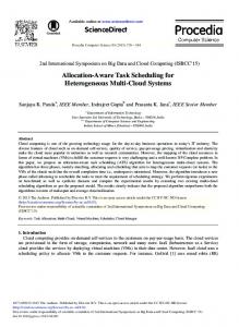
Fig. 1. System model of DAG scheduling service on clouds [4].

3. Problem definition 3.1. System model As illustrated in Fig. 1, the system model for the scheduling problem on cloud environments includes three layers: the task graph, the resource graph, and the cloud infrastructure layers [4, 31]. The task graph layer comprises of tasks with precedence constraints that users submit for executing complex applications. The resources graph layer represents a network of virtual machines (VMs), and the cloud infrastructure layer consists of interconnected physical computer nodes. According to [7], task placement is to find a placement of processors for executing a task, which is similar to the processor allocation. Task scheduling is to determine the placement and starting time of tasks. When time dimension is added to a placement algorithm, the algorithm is extended to a scheduling algorithm and is also regarded as a 3D placement algorithm. This study aims to provide a DAG task scheduling service on a cloud computing system, including the processor allocation and the determination of the start time of tasks on processors. The targeted computing platform is composed of a set of heterogeneous processors that provide  services of different capabilities and costs [10]. Let P = p1 , p2 , . . . , p|P | as the processor set, where |P | represents the size of set P. For any set X , this study uses |X | to denote its size. A parallel application running on processors is represented by the DAG G = {N , E , C , W }. N represents a set of nodes in G, and ni ∈ N represents a task with different execution times on different processors. E is a set of communication edges, and each edge ei,j ∈ E represents a communication message (i.e., transferred data or time) from task ni to task nj . Accordingly, C is the set of communication edges, and ci,j represents the communication message (i.e., the time) between ni and nj if they are not assigned to the same processor. W is an |N | × |P | matrix, where wi,k denotes the execution time of task ni running on processor pk . pred(ni ) represents the set of immediate predecessors of task ni , and succ (ni ) represents the set of immediate successors of task ni . In a given DAG, the task without a predecessor is the entry task denoted as nentry , and the task without any successor is the exit task denoted as nexit . If a DAG has multiple nentry or nexit tasks, a dummy

Fig. 2. A DAG-based sample with ten tasks [6].

Table 1 Execution time of tasks on different resources in Fig. 2 [6]. ni

p1

p2

p3

1 2 3 4 5 6 7 8 9 10

14 13 11 13 12 13 7 5 18 21

16 19 13 8 13 16 15 11 12 7

9 18 19 17 10 9 11 14 20 16

entry or exit task with zero-weight dependencies is added to the graph. Fig. 2 shows a motivating example of a DAG-based parallel application with 10 tasks. Table 1 provides the execution times of tasks on three processors {p1 , p2 , p3 }. As shown in Fig. 2, the weight 12 of the edge between n1 and n3 represents the communication time denoted as c1,3 = 12 if n1 and n3 are not assigned to the same processor. As indicated in Table 1, the execution time of task n1 on processor p1 is 14, denoted as w1,1 = 14. The same task has different execution times on different resources because of the heterogeneity of processors.

4

W. Chen et al. / Future Generation Computer Systems 74 (2017) 1–11 Table 2 Mathematical notations in this paper.

3.2. Cost model The cost model is based on a pay-as-you-go condition, and the users are charged according to the amount of time that they have used processors. Each processor has an individual unit price because processors in the system are completely heterogeneous. We assume that pricek is the unit price of the allocated computing service on processor pk . All computation and storage services are assumed to be in the same physical region. Hence, communication time ci,j only depends on the amount of data to be transferred between task ni and task nj and is independent of the computation service on the processors [21]. The only exception is when both tasks ni and nj are executed on the same processor, where ci,j = 0. Furthermore, the internal data transfer cost is free in most actual applications, so the data transfer cost is assumed to be zero in our model. Accordingly, we formally define the cost costi,k of task ni on processor pk and total cost cost (G) of a DAG as follows: costi,k = cost (ni , pk ) = wi,k × pricek , cost (G) =

|N | 

wi,f (i) × pricef (i) ,

(1) (2)

i =1

where f (i) is the index of the processor assigned to task ni , wi,f (i) is the execution time of task ni on processor f (i), pricef (i) is the unit price of processor pf (i) . 3.3. Budget constraint

costmin (G) =

|N | 

costmin (ni ),

(3)

costmax (ni ),

(4)

i=1

respectively. Assuming that the budget constraint of an application is costbud (G), then it should be larger than or equal to costmin (ni ) and less than or equal to costmax (ni ); otherwise, costbud (G) is not always satisfied. Hence, this study assumes that costbud (G) belongs to the scope of costmin (ni ) and costmax (ni ), that is, costmin (G) ≤ costbud (G) ≤ costmax (G).

(5)

3.4. Problem formulation This study addresses the task scheduling problem of assigning an available processor with a proper price for each task while minimizing the schedule length of the application and ensuring that the total cost of the application does not exceed the budget constraint. The formal description is finding the processor and budget assignments for all tasks with the objective of minimizing the schedule length of the application, SL(G) = AFT (nexit ), where AFT (nexit ) represents the actual finish time (AFT) of the exit task, subject to its budget constraint: cost (G) =

|N | 

Execution time of task ni running on processor pk Communication time between ni and nj Set of immediate predecessors of task ni Set of immediate successors of task ni Upward rank value of tasks Index of the processor assigned to task ni Unit price of processor pk cost (ni , pk ), cost of task ni on processor pk , Minimum cost of executing task ni Maximum cost of executing task ni Minimum cost of the application G Maximum cost of the application G Budget constraint of the application G Total cost of the application G Schedule length of the application G Budget level of an application Cost of unassigned task ni Budget constraint of task ni Spare budget of task ni

ci,j pred(ni ) succ (ni ) ranku f (i) pricek costi,k costmin (ni ) costmax (ni ) costmin (G) costmax (G) costbud (G) cost (G) SL(G) bl costbl (ni ) costbud (ni ) ∆cost (ni )

Table 3 Upward rank values for tasks in Fig. 2 [6]. ni

n1

n3

n4

n2

n5

n6

n9

n7

n8

n10

ranku (ni )

108

80

80

77

69

63

44

43

36

15

We first need to set the priority of task assignment before assigning tasks to processors. Similar to [11,12], we employ ranku of a task as the common task priority standard: ranku (ni ) = wi + max {ci,j + ranku (nj )}, nj ∈succ (ni )

i=1

costmax (G) =

Definition

wi,k

3.5. Task prioritization

As the execution time of each task on processors is known, the minimum and maximum costs of task ni , denoted by costmin (ni ) and costmax (ni ), respectively, can be obtained by traversing all the processors. For the total cost of the application, G is the sum of that of each task, the minimum and maximum costs of a DAG are: |N | 

Notation

cost (ni , pf (i) ) ≤ costbud (G).

(6)

i =1

Table 2 shows the mathematical notations used in this paper.

where wi is the average execution time of task ni on processors  |P | and calculated as wi = k=1 wi,k / |P |. It represents the length of the longest path from task ni to the exit node nexit , including the communication time between tasks and execution time of tasks. For the exit task, ranku (nexit ) = wexit . Table 3 shows the upward rank values of all tasks in Fig. 2. Note that, as observed from Table 3, the task priority by the decreasing order of ranku is {n1 , n3 , n4 , n2 , n5 , n6 , n9 , n7 , n8 , n10 }. 4. Minimizing schedule length with budget constraints In this section, the algorithm for minimizing the schedule length using the budget level (MSLBL) is presented, which aims to find a fair schedule policy for minimizing the schedule length of budget constrained applications with low complexity and high performance on heterogeneous cloud computing systems. Such problem is decomposed into two sub-problems, namely, satisfying the budget constraint and minimizing the schedule length. We first solve these two sub-problems separately, and then present the algorithm by integrating the two sub-problems. 4.1. Existing HBCS algorithm Before the MSLBL algorithm is presented, we analyze the existing algorithm HBCS. Considering that users consume services based on their QoS requirements and minimizing the schedule length of budget constrained applications is one of the most important concerns, the state-of-the-art HBCS [11] is proposed by presupposing the unassigned tasks with the minimum execution cost while still satisfying the budget constraint of the application. The objective of HBCS is to quantitatively select the processor


5

Fig. 3. Scheduling of the application in Fig. 2 with costbud (G) = 500 using HBCS [11]. Table 5 Task assignment of the application in Fig. 2 with costbud (G) = 500 using HBCS [11].

Table 4 Unit price of processors in Fig. 2. pk

pricek

ni

∆ cos t

costbud (ni )

AST (ni )

AFT (ni )

f (n i )

costi,f (ni )

p1 p2 p3

3 5 7

1 3 4 2 5 6 9 7 8 10

126 26 25 25 25 1 1 1 1 1

189 159 65 64 61 64 55 22 16 36

0 9 18 27 40 28 52 70 77 94

9 28 26 40 52 37 70 77 82 101

P3 P3 P2 P1 P1 P3 P1 P1 P1 P2

63 133 40 39 36 63 54 21 15 35

with the highest worthiness value for tasks by the descending order of ranku and minimize the schedule length of the application under the user’s specified budget constraint. The core details are explained as follows: (1) HBCS first invokes the HEFT algorithm on all the processors and obtains costHEFT (G) and costmin (G). (2) HBCS compares costHEFT (G) with costbud (G). If costbud (G) is larger than or equal to costHEFT (G), it returns the schedule map assigned by HEFT. (3) HBCS preassigns each task with the minimum execution cost and initializes the parameters, then traverses all processors for all tasks by the descending order of ranku . It determines the processor for tasks by calculating the parameters FT (ni , pk ), Cost (ni , pk ), CostCoeff , w orthiness(ni , pk ) and RB. (4) HBCS assigns tasks to the processor with the highest worthiness value and returns the schedule map. For convenience of description, we define the spare budget to observe the budget assignment of tasks in applications on heterogeneous cloud computing systems. Definition 1 (Spare Budget). Spare budget is defined as the difference between the budget constraint of a task and its preassigned cost, as shown in Eq. (7):

∆cost (ni ) = costbud (ni ) − costpre (ni ),

(7)

where costbud (ni ) is the budget constrained cost of task ni , costpre (ni ) is the preassigned cost of the unassigned task ni . Initially, the spare budget of application G is the difference between costbud (G) and costpre (G). We illustrate the motivating parallel application to explain the HBCS algorithm. We set the budget constraint of G as costbud (G) = 500. We assume that the unit price of processors in Fig. 2 is known, as shown in Table 4. We compute the minimum cost value of the application as costmin (G) = 353 using Eq. (6). Table 5 shows the task assignment of the parallel application in Fig. 2 using HBCS, where all tasks satisfy their individual budget constraints. The actual execution cost of the application is cost (G) = 499, and its schedule length is SL(G) = 101. Fig. 3 also shows the scheduling of the parallel application G in Fig. 2 with costbud (G) = 500 using HBCS. Note that the arrows in Fig. 3 represent the generated communication times between tasks. This example verifies that the use of HBCS can ensure that the actual cost of the application does not exceed the user given

cost (G) = 499 ≤ costbud (G), SL(G) = 101.

budget constraint, that is, cost (G) ≤ costbud (G). However, as shown in Table 5, the task with higher priority has more spare budget than those with low priorities. The potential reason for this is that HBCS presupposes unassigned tasks in the application with the minimum execution cost and the spare budget of the application is shared by the former assigned tasks that have more opportunities. Thus, the task with low priority tends to select processors with minimum costs but long execution times, which may result in a longer schedule length of the application. As shown in Table 5, tasks n6 to n10 have few spare budget available. It is unfair for tasks with low priority. Thus, the HBCS algorithm should be further optimized. 4.2. Satisfying budget constraint Assuming that the task to be assigned is ns (j) , where s(j) represents the jth assigned task, then {ns(1) , ns (2) , . . . , ns(j−1) } represents the task set where the tasks have been assigned, and {ns(j+1) , ns (j+2) , . . . , ns(|N |) } represents the task set where the tasks have not been assigned. Initially, all tasks of the application are unassigned. To ensure fairness for all tasks as much as possible, we first provide the definition of the global level [4]. Definition 2 (Budget Level). Budget level is defined as the ratio of the difference between costbud (G) and the minimum execution cost of the application to the difference between the maximum and minimum execution costs of application G, as shown in Eq. (8): bl =

costbud (G) − costmin (G) costmax (G) − costmin (G)

.

(8)

According to Eqs. (5) and (8), we have bl ∈ [0, 1]. Note that, the original bl is only applied to homogeneous cloud computing systems [4]. In this study, we make bl be suitable for heterogeneous systems by transferring the budget constraint of an application into budget constraints of tasks and complete scheduling based on EFT. The workflow model in [4] does not consider the communication

6


time between tasks. However, we consider both the precedence constraint and the communication time between tasks in our application model. Last but not least, we give the proof of converting the budget constraint of an application into budget constraints of tasks using the budget level. Then, we preassign unassigned tasks with a budget level cost described as:

Second, we assume that the jth task ns(j) can find an assigned processor pf (s(j)) to satisfy costbud (G), and we have: costns (j) (G) =

(9)

costmin (ns(j) ) ≤ costpre (ns(j) ) ≤ costmax (ns(j) ).

costbl (ns(i) ).

Theorem 1. Each task in the parallel application G can always find an assignment of processors to satisfy: j−1 

Hence, j 

costs(i),f (s(i)) ≤ costbud (G) −

(11)

(16)

Finally, for the (j + 1)th task, the execution cost of an application is costns (j+1) (G) =

j 

costs(i),f (s(i)) + costs(j+1),f (s(j+1))

i=1

|N | 

costbl (ns(i) ) ≤ costbud (G).

(17)

costns (j+1) (G) ≤ costbud (G) −

|N | 

costbl (ns(i) )

i=j+1

Proof. We use the mathematical induction to prove it. First, for the entry task n1 = ns(1) , all tasks are not assigned to processors: costns (1) (G) = costs(1),pk +

|N | 


(12)

i =2

According to Eqs. (8), (9) and (12), we have |N | 

|N | 

costbl (ns(i) )

|N | 

costbl (ns(i) )

i=j+2

= costbud (G) − costbl (ns(j+1) ) + costs(j+1),f (s(j+1)) .

(18)

When ns(j+1) is assigned a cost in range of costmin (ns(j+1) ) to costbl (ns(j+1) ), we have: (19)

According to Eq. (10), ns(j+1) can at least be assigned to the processor with the minimum cost, that is, ns(j+1) can also find an assigned processor to satisfy costbud (G). When all tasks can find individual assigned processors to satisfy costbud (G), Theorem 1 is satisfied. This completes the proof.

costbl (ns(i) ) − costbl (ns(1) )

i=1

|N | 

+ costs(j+1),f (s(j+1)) +

costns (j+1) (G) ≤ costbud (G).

i=2

= costs(1),pk +

costbl (ns(i) ).

i=j+1

i=j+1

= costs(1),pk +

|N | 

Known as Eqs. (13) and (14), we have:


costns(1) = costs(1),pk +


i=j+1

i =j +2

costs(i),f (s(i)) + costs(j),pk

|N | 

|N | 

costs(i),f (s(i)) +

i =1

+

i =1

+

j 

i=1

For any task ns (j) , the actual execution cost cos(G) should be less than or equal to costbud (G) only if costns (j) (G) ≤ cos tbud (G). Its proof is provided in the following.

costns (j) (G) =

costns (j) (G) =

i=j+1

i=1

(15)

such that,

(10)

Hence, when assigning ns (j) , the total cost of the application G is calculated as: costs(i),f (s(i)) + cs(j),pk +


i=j+1

Correspondingly, costpre (ns(j) ) in Eq. (7) is equal to costbl (ns(j) ). According to Eqs. (8) and (9):

costns (j) (G) =

|N | 

+

− costmin (ns(j) )) × bl.

|N | 

costs(i),f (s(i)) + costs(j),f (s(j))

i =1

costbl (ns(j) ) = costmin (ns(j) ) + (costmax (ns(j) )

j −1 

j−1 

costmin (ns(i) )

4.3. Minimizing schedule length

i=1

+

 |N | 

costmax (ns(i) ) −

i=1

|N | 

 costmin (ns(i) )

i=1

× bl − costbl (ns(1) ) = costs(1),pk + cos tbud (G) − costbl (ns(1) )

(13)

Namely, Eq. (13) should be satisfied costs(1),pk + cos tbud (G) − costbl (ns(1) ) ≤ cos tbud (G).

(14)

According to Eq. (10), costbl (ns(1) ) is larger than or equal to costmin (ns(1) ), that is, the processor with the minimum execution cost can be assigned to task ns(1) at the least. Hence, ns(1) can find an assigned resource to satisfy Eq. (14), that is, Eq. (11) is satisfied for ns(1) .

HEFT is a well-known precedence-constrained task scheduling, which is based on the DAG model to reduce schedule length to a minimum combined with low complexity and high performance in heterogeneous systems [6,22]. Task prioritization is based on upward rank value (ranku ) and task assignment is based on the earliestfinishtime.   EST nj , pk and EFT nj , pk denote the earliest start time (EST) and EFT of task nj on processor pk , respectively, defined as: EST (nj , pk ) = max{Tav ail(pk ) , max {AFT (ni ) + ci,j }},

(20)

EFT (nj , pk ) = EST (nj , pk ) + wj,k ,

(21)

ni ∈pred(nj )

where Tav ail(pk ) is the earliest time at which the processor pk is ready for task execution. Communication time ci,j is zero if nj and


its predecessor ni are assigned to the same resource. For the entry task, EST (nentry , pk ) = 0. AST (ni ) and AFT (ni ) are the actual start time and the actual finish time of task ni , respectively. To select the best suitable processor, the cost and time tradeoff is evaluated. Typically, the faster the speed of processors is, the higher the execution cost of tasks is. However, this is not always the case on heterogeneous computing systems. After transferring the budget constraint of applications to that of each task, tasks are assigned to processors with the minimum EFT by using the insertion-based scheduling strategy while satisfying the budget constraint of tasks. 4.4. Proposed MSLBL algorithm We first give the budget constraint of each task before we propose the algorithm. According to Eq. (11), we have: costs(j),f (s(j)) ≤ costbud (G) −

j −1 

costs(i),f (s(i)) −

i=1

|N | 

costbl (ns(i) ).

i=j+1

Hence, let the budget constraint of task ns (j) be costbud (ns(j) ) = costbud (G) −

j −1 

costs(i),f (s(i))

i=1

−

|N | 

costbl (ns(i) ).

(22)

i=j+1

Then, the budget constraint of the application can be transferred to that of each task. That is, we just let ns (j) satisfy the following constraint: costs(j),f (s(j)) ≤ costbud (ns(j) ). Hence, when assigning the task ns(j) , we can directly consider the budget constraint costbud (ns(j) ) of ns(j) and do not have to be concerned about the budget constraint costbud (G) of the application G. In this way, a low time complexity heuristic algorithm can be obtained. Inspired by the above analysis, we propose the MSLBL algorithm to minimize the schedule length while still satisfying the budget constraint of the application. The steps of MSLBL are described in Algorithm 1. The main idea of MSLBL is that the budget constraint of the application is transferred to that of each task to change the budget constraint of each task by using the budget level. The algorithm assigns processors to tasks by the descending order of ranku values, and each task select the processor with the minimum EFT while satisfying its individual budget-level constraint. The core details are explained as follows: (1) In Lines 1–6, the minimum cost value of G and budget level cost of tasks are computed. (2) In Lines 7–9, the possibility of finding a schedule under the user provided budget constraint is verified. (3) In Lines 10–23, the algorithm starts to map the tasks of the application to processors. At each step, the task with the highest priority among the unscheduled tasks is selected as the current task ns (j) , and its budget constraint is set. Next, for task ns (j) , the processor that satisfies its budget level constraint and has the minimum EFT is selected. After assigning the processor to ns (j) , the spare budget ∆ cos t is updated using Eq. (7) and the for loop is broken. (4) In Lines 24–25, the actual execution cost and final schedule length SL(G) are computed. In terms of time complexity, MSLBL requires the computation of ranku and the minimum and maximum costs of the application that has complexity O(|N |×|P |). In the processor selection phase for the current task, the complexity is O(|N | × |P |) for computing EFT, and O(|P |) for selecting the resource with the minimum EFT, satisfying its budget constraint. The total time is O(|N | × |P | + |N | · (O(|N | × |P |) + |P |, where time complexity is of the order O(|N |2 × |P |).

7

Algorithm 1 The MSLBL Algorithm Input: G = {N , E , C , W }, for ∀j, pj ∈ P , pricej , costbud (G) Output: SL(G), cost (G) 1: Sort the tasks in a list dlist by descending order of ranku values; 2: for (∀i, ni ∈ N) do 3: Compute costmin (ni ) and costmax (ni ). 4: end for 5: Compute costmin (G) and costmax (G) using Eqs. (3) and (4); 6: Compute bl, costbl (ni ) and ∆cost (ni ) using Eqs. (7), (8) and (9), respectively; 7: if (costbud (G) ≤ costmin (G)) then 8: return 0; 9: end if 10: while (there are tasks in dlist) do 11: ns(j) = dlist.out(); 12: Compute costbud (ns(j) ) using Eq. (22); 13: for (∀k, pk ∈ P) do 14: Compute costs(j),k and EFT (ns(j) , pk ) using Eq. (21); 15: end for 16: for (k = 1; i ≤ |P | ; k + +) do 17: if (costs(j),k ≤ costbud (ns(j) )) then 18: Select the processor with the minimum EFT for task ns(j) ; 19: Update ∆cost using Eq. (7); 20: AFT(ns(j) ) = EFT (ns(j) , pk ); 21: end if 22: end for 23: end while 24: Compute the actual cost cost (G) using Eq. (2); 25: Compute SL(G) = AFT (nexit ); 26: return SL(G), cost (G).

Table 6 Task assignment of the application in Fig. 2 with costbud (G) = 500 using MSLBL. ni

∆ cos t

costbud (ni )

AST (ni )

AFT (ni )

f (n i )

costi,f (ni )

1 3 4 2 5 6 9 7 8 10

0 8 30 46 65 0 17 35 48 65

50 63 86 104 70 80 95 69 80 112

0 14 23 25 25 35 54 38 59 75

14 25 31 38 35 44 66 45 64 82

P1 P1 P2 P1 P3 P3 P2 P1 P1 P2

42 33 40 39 70 63 60 21 15 35

cost (G) = 418 ≤ costbud (G), SL(G) = 82.

4.5. Example of the MSLBL algorithm We present an motivating example to show the results using the MSLBL algorithm. We consider the condition costbud (G) = 500 for the application in Fig. 2, and the unit price of processors is shown in Table 4. Table 6 shows the task assignment of the parallel application in Fig. 2 with costbud (G) = 500 using MSLBL. The total cost of the application is 418 and its schedule length is 82, which is less than that using the HBCS algorithm. Fig. 4 shows the scheduling of the parallel application G in Fig. 2 with costbud (G) = 500 using MSLBL. 5. Experimental results and discussion This section presents performance comparisons of the MSLBL algorithm with HBCS [11] and DBCS [12] algorithms because they have the similar application models. 5.1. Experimental metrics We resort to simulation method to verify our algorithms. We implement a simulator in Java language. All simulative experiments are conducted on a PC platform with an Intel Core i5 2.60 GHz CPU and 4 GB memory. The simulated heterogeneous cloud computing system contains 128 processors with different computing abilities and unit prices, where the types and the prices of processors are based on the Amazon Elastic Compute Cloud (EC2) environment [32]. The application and processor parameters

8


Fig. 4. Scheduling of the application in Fig. 2 with costbud (G) = 500 using MSLBL. Table 7 Actual cost and schedule length of Fast Fourier transform applications with budget constraints for varying number of tasks.

|N | 96 224 512 1152 2560

costmin (G)

40 76 221 463 770

costbud (G)

48 91 265 556 924

HBCS [11]

|N |

MSLBL

cost (G)

SL(G)

cost (G)

SL(G)

48 91 265 556 924

796 1 302 13 945 25 637 31 991

47 90 265 556 924

739 984 9 967 15 222 22 401

are: 0.01 $/h ≤ pricek ≤ 1 $/h, 0.01 h ≤ wi,k ≤ 128 h, 0.01 h ≤ ci,j ≤ 30 h. The number of tasks can be dynamically set and varies between 10 and 2627 in our experiments. The average bandwidth between the computation services is set to 20 MBps which is the approximate average bandwidth of the computation services (EC2) in Amazon [5]. The number of tasks executed on each processor is determined by the scheduling algorithm. The performance metrics selected for comparison are the actual cost cost (G), the final schedule length SL(G) of budget constrained applications, and the acceptance ratio (AR) of budget and deadline constrained applications. The AR is expressed by Eq. (23): AR =

number of acceptance total number of experiments

.

Table 8 Actual cost of the Fast Fourier transform application with ρ = 256 (i.e.,|N | = 2560) for varying budget constraints.

(23)

To verify the effectiveness of the scheduling algorithms, real applications with precedence constrained tasks are widely used in some high-performance computing, such as Fast Fourier transform and Gaussian elimination [6]. We use these two types of real parallel applications under the condition of the budget and budgetdeadline constraints to observe the results. 5.2. Fast Fourier transform parallel applications A new parameter ρ is used as the size for the Fast Fourier transform application, and the number of tasks is |N | = 2 × ρ−1+ρ × log2 ρ , where ρ = 2y for some integer y. Fig. 5 shows an example of the Fast Fourier transform parallel applications with ρ = 8. Note that ρ exit tasks exist in this application with size ρ . To adapt the application of this study, we create a dummy exit task with zero execution time, which connects these ρ exit tasks with zero communication time. 5.2.1. Varying number of tasks This experiment is conducted to compare the actual cost and final schedule lengths of Fast Fourier transform parallel applications for varying number of tasks. We limit costbud (G) as costmin (G) × 1.2. The number of tasks is changed from 96 (small scale) to 2560 (large scale) when ρ is changed from 16 to 256. As shown in Table 7, the budget constraints and actual costs of the applications increase gradually with the number of tasks. At

2560 2560 2560 2560 2560

costmin (G)

923 923 923 923 923

costbud (G)

1015 1107 1200 1292 1384

HBCS [11]

MSLBL

cost (G)

SL(G)

cost (G)

SL(G)

1015 1107 1200 1292 1384

48 321 48 319 48 292 48 235 48 235

1015 1107 1200 1292 1384

35 134 2 9178 25 428 21 404 19 794

the same time, the actual cost of applications in different scales using HBCS and MSLBL satisfy the budget constraints. Such results verify that these algorithms can satisfy the budget constraints of applications in practice. In addition to satisfying the budget constraints of the applications, an exciting phenomenon is that MSLBL can generate shorter schedule length than HBCS in different scale parallel applications. Furthermore, the difference becomes more and more obvious with the increase of the number of tasks. For example, when |N | = 2560, the schedule length using MSLBL is 22401, which is 70% of 31 991 that used HBCS. Such results indicate that MSLBL is very suitable for minimizing schedule length of budget constrained parallel applications and is useful for different scale parallel applications. 5.2.2. Varying budget constraints To observe the performance in different scales of applications, this experiment is conducted to compare the actual cost and final schedule length of Fast Fourier transform parallel applications for varying budget constraints. We limit the size of the application as ρ =256 (i.e.,|N | = 2560). costbud (G) is changed from costmin (G)×1.1 to costmin (G) × 1.5. Table 8 shows that the actual costs of applications using HBCS and MSLBL can satisfy the budget constraints in all cases. In addition, the schedule length using MSLBL is less than those of the HBCS algorithm. Furthermore, the difference in the schedule lengths using the two algorithms becomes more and more obvious with the increasing budget constraints of the application. For example, when costbud (G) is costmin (G) × 1.1, the schedule lengths using MSLBL is 35 134, 73% of that using HBCS, whereas that using MSLBL is 19 794 and 41% of that using HBCS when costbud (G) is costmin (G) × 1.5 in this experiment. 5.3. Gaussian elimination parallel applications To verify the performance further, this experiment uses another important real parallel application (i.e., Gaussian elimination) as experimental object. A new parameter ρ is used as the matrix size of the Gaussian elimination application, and the total number of ρ 2 +ρ−2

tasks is |N | = [6]. Fig. 6 shows an example of the Gaussian 2 elimination parallel application with ρ = 5.


9

Fig. 5. Example of fast Fourier transform parallel applications with ρ = 8. Table 10 Actual cost and schedule length of Gaussian elimination parallel applications with ρ = 72 (i.e., |N | = 2627) for varying budget constraints.

|N | 2627 2627 2627 2627 2627

Fig. 6. Example of the Gaussian elimination parallel application with ρ = 5. Table 9 Actual cost and schedule length of Gaussian elimination applications with budget constraints for varying numbers of tasks.

|N | 77 299 665 1175 1829 2627

costmin (G)

25 168 230 439 629 2142

costbud (G)

30 201 275 527 755 2570

HBCS [11]

MSLBL

cost (G)

SL(G)

cost (G)

SL(G)

30 201 275 527 754 2570

1 506 3 520 12 977 21 436 33 903 35 460

30 201 275 526 754 2569

1 506 3 341 8 797 16 409 25 076 22 389

5.3.1. Varying number of tasks To observe the performance in different scales of real applications further, this experiment is conducted to compare the actual costs and final schedule length of Gaussian elimination parallel applications for varying number of tasks. We limit costbud (G) as costmin (G) × 1.2. The number of tasks is changed from 77 (small scale) to 2627 (large scale) when ρ is changed from 12 to 72, which are approximately equal to the numbers of the Fast Fourier transform application in experiment 5.2.1.

costmin (G)

1026 1026 1026 1026 1026

costbud (G)

1129 1232 1334 1437 1540

HBCS [11]

MSLBL

cost (G)

SL(G)

cost (G)

SL(G)

1129 1232 1334 1437 1540

61 297 61 359 61 096 61 058 60 819

1129 1231 1334 1436 1540

50 800 46 711 44 497 40 957 38 934

Table 9 shows the results of the Gaussian elimination applications for varying numbers of tasks using two algorithms. The actual cost and schedule length of applications increase with the increase of the number of tasks. However, the schedule length in Gaussian elimination parallel applications is longer than that in Fast Fourier transform parallel applications. Such results indicate that the Fast Fourier transform application has better parasitism than the Gaussian elimination application in the structure, and can generate shorter schedule length. Similar to the results of Experiment 5.2.1, the actual costs of applications using HBCS and MSLBL can still satisfy and are close to the budget constraints of Gaussian elimination applications in different scales. The schedule length using MSLBL is shorter than that using HBCS in large-scale applications. For example, when the task number exceeds 600, the schedule lengths using MSLBL is 22 389, while that using HBCS are 35 460. The former is merely 63.1% of the latter. Such results indicate that MSLBL can satisfy the budget constraints with the minimum schedule length and generate shorter schedule lengths than HBCS for large-scale Gaussian elimination applications. 5.3.2. Varying budget constraints This experiment is conducted to compare the actual cost and the final schedule length of Gaussian elimination parallel applications for varying budget constraints. We limit the size of the application as ρ = 72 (i.e.,|N | = 2627), which is approximately equal to the number of tasks of the Fast Fourier transform parallel application in Experiment 5.2.2. costbud (G) is changed from costmin (G) × 1.1 to costmin (G) × 1.5. Table 10 shows the results of the Gaussian elimination parallel application for varying budget constraints using the two algorithms. Similar to the results of Table 8 for Experiment 5.2.2,

10


Table 11 Acceptance ratio of the Fast Fourier transform applications with budget-deadline constraints for varying numbers of tasks.

Table 12 Acceptance ratio of the Gaussian elimination parallel applications with budgetdeadline constraints for varying numbers of tasks.

|N |

HBCS [11]

DBCS[12]

MSLBL

|N |

HBCS [11]

DBCS [12]

MSLBL

96 224 512 1152 2560

71% 66% 36% 10% 0%

73% 67% 36% 10% 0%

87% 82% 64% 37% 15%

77 299 665 1175 1829 2627

77% 84% 77% 62% 60% 47%

88% 84% 77% 62% 60% 47%

89% 89% 81% 83% 88% 73%

the schedule length using MSLBL is shorter than that using HBCS in the same scale levels. When costbud (G) is costmin (G) × 1.5, the schedule lengths using HBCS and MSLBL are 60 819 and 38 934, respectively. The latter is 64% of the former. The actual costs using two algorithms are within the budget constraints in all cases. The overall trend of both Gaussian elimination and Fast Fourier transform applications in the same scale is similar. That is, MSLBL has the shorter schedule length than HBCS for budget constrained parallel applications. Such results indicate that MSLBL is more effective in different types of parallel applications than the stateof-the-art algorithm. 5.4. Verification of budget-deadline constrained scheduling The proposed approach is verified further by experiments of budget-deadline constrained parallel applications. For the problem of budget and deadline constrained scheduling, a scheduling can be accepted only if its actual cost and schedule length of the application can satisfy the budget and deadline constraints, respectively. DBCS is used to obtain a feasible scheduling by considering the budget and deadline constraints of the application simultaneously. HBCS and the proposed algorithm (i.e., MSLBL) are used to minimize the schedule length while satisfying the budget constraint of the application. This experiment is conducted to compare the AR of Fast Fourier transform and Gaussian elimination parallel applications for varying number of tasks. We limit the size of applications changed from 96 (small scale) to 2560 (large scale) when ρ is changed from 16 to 256 in the Fast Fourier transform applications, and changed from 77 (small scale) to 2627 (large scale) when ρ is changed from 12 to 72 in the Gaussian elimination parallel applications. The budget constraint of applications costbud (G) is considered in the range of costmin (G) × 1.1 to costmin (G) × 10. The deadline constraint of applications is defined in the range of SLHEFT (G) × 1.1 to SLHEFT (G) × 10, where SLHEFT (G) is the schedule length of an application using the HEFT algorithm. The total number of experiments is 1000. Table 11 shows that the AR using the three algorithms decreases with the increase of the number of tasks in the Fast Fourier transform applications. However, the AR using MSLBL is significantly higher than those using HBCS and DBCS in the same scale. For example, when |N | = 1152, the AR using MSLBL and HBCS are 37% and 10%, respectively. An interesting phenomenon is that the ARs obtained by using HBCS and DBCS are almost the same. This is mainly because these two algorithms adopt the preassignment scheme with the minimum execution cost of tasks. Compared with the results in Table 11, the change trend of the AR of Gaussian elimination applications in Table 12 is similar to that of Fast Fourier transform applications. However, the ARs using the three algorithms change slowly with the increase of the number of tasks. The AR using MSLBL is higher than those using HBCS and DBCS, and the difference between them increases with the increase of the number of tasks. The ARs using HBCS and DBCS are roughly the same in the same scale levels. The results indicate that MSLBL obtains the minimum schedule length under budget

and deadline constraints and has a better acceptance rate than the other two algorithms. The combination of all the results of Fast Fourier transform and Gaussian elimination parallel applications with budget and budget-deadline constraints indicates that the proposed MSLBL algorithm is very effective in schedule length minimization while satisfying the budget constraints. 6. Conclusions An algorithm of schedule length minimization MSLBL for budget constrained parallel applications on heterogeneous cloud computing systems is developed in this study. First, the proposed algorithm can always satisfy the budget constraint, and the correctness is verified using proof and experiments. Second, the proposed MSLBL algorithm implements efficient and low time complexity task scheduling to minimize the schedule length. The MSLBL algorithm using the budget-level design technique is highly efficient in satisfying the budget constraint and minimizing the schedule length of different scales of real parallel applications compared with the existing budget and budgetdeadline constrained algorithm. The proposed MSLBL algorithm could effectively improve part of the cost-aware design for parallel applications on heterogeneous cloud computing systems. Acknowledgments This work is partially supported by the National Natural Science Foundation of China with Grant No. 61672217, 61602164, the China Postdoctoral Science Foundation under Grant No. 2016M592422. References [1] M.W. Convolbo, J. Chou, Cost-aware DAG scheduling algorithms for minimizing execution cost on cloud resources, J. Supercomput. 72 (3) (2016) 985–1012. [2] Y. Kong, M. Zhang, D. Ye, A belief propagation-based method for task allocation in open and dynamic cloud environments, Knowl.-Based Syst. 115 (2017) 123–132. [3] J. Broberg, S. Venugopal, R. Buyya, Market-oriented grids and utility computing: The state-of-the-art and future directions, J. Grid Comput. 6 (3) (2008) 255–276. [4] C.Q. Wu, X. Lin, D. Yu, et al., End-to-end delay minimization for scientific workflows in clouds under budget constraint, IEEE Trans. Cloud Comput. 3 (2) (2015) 169–181. [5] Z. Wu, X. Liu, Z. Ni, et al., A market-oriented hierarchical scheduling strategy in cloud workflow systems, J. Supercomput. 63 (1) (2013) 256–293. [6] H. Topcuoglu, S. Hariri, M. Wu, Performance-effective and low-complexity task scheduling for heterogeneous computing, IEEE Trans. Parallel Distrib. Syst. 13 (3) (2002) 260–274. [7] X. Zhou, Y. Wang, X. Huang, C. Peng, Fast on-line task placement and scheduling on reconfigurable devices., in: FPL, 2007, pp. 132–138. [8] M.A. Rodriguez, R. Buyya, Deadline based resource provisioning and scheduling algorithm for scientific workflows on clouds, IEEE Trans. Cloud Comput. 2 (2) (2014) 222–235. [9] S. Abrishami, M. Naghibzadeh, D.H.J. Epema, Cost-driven scheduling of grid workflows using partial critical paths, IEEE Trans. Parallel Distrib. Syst. 23 (8) (2012) 1400–1414. [10] F. Wu, Q. Wu, Y. Tan, et al., PCP-B2 : Partial critical path budget balanced scheduling algorithms for scientific workflow applications, Future Gener. Comput. Syst. 60 (2016) 22–34.

W. Chen et al. / Future Generation Computer Systems 74 (2017) 1–11 [11] H. Arabnejad, J.G. Barbosa, A budget constrained scheduling algorithm for workflow applications, J. Grid Comput. 12 (4) (2014) 665–679. [12] H. Arabnejad, J.G. Barbosa, R. Prodan, Low-time complexity budget-deadline constrained workflow scheduling on heterogeneous resources, Future Gener. Comput. Syst. 55 (2016) 29–40. [13] M. Malawski, G. Juve, E. Deelman, et al., Algorithms for cost-and deadlineconstrained provisioning for scientific workflow ensembles in iaasclouds, Future Gener. Comput. Syst. 48 (2015) 1–18. [14] T.C. Hu, Parallel sequencing and assembly line problems, Oper. Res. 9 (6) (1961) 841–848. [15] G. Xie, G. Zeng, L. Liu, R. Li, K. Li, High performance real-time scheduling of multiple mixed-criticality functions in heterogeneous distributed embedded systems, J. Syst. Archit. (2016) 1–13. [16] S. Abrishami, M. Naghibzadeh, D.H.J. Epema, Deadline-constrained workflow scheduling algorithms for infrastructure as a service clouds, Future Gener. Comput. Syst. 29 (1) (2013) 158–169. [17] Q. Huang, S. Su, J. Li, P. Xu, K. Shuang, X. Huang, Enhanced energy-efficient scheduling for parallel applications in cloud, in: Proceedings of the 2012 12th IEEE/ACM International Symposium on Cluster, Cloud and Grid Computing, (ccgrid 2012), IEEE Computer Society, 2012, pp. 781–786. [18] X. Xiao, G. Xie, R. Li, K. Li, Minimizing schedule length of energy consumption constrained parallel applications on heterogeneous distributed systems. in: 14th IEEE International Symposium on Parallel and Distributed Processing with Applications, ISPA 2016, 2016, pp. 1471–1476. [19] L. Yang, J. Cao, S. Tang, N. Suri, Run time application repartitioning in dynamic mobile cloud environments, IEEE Trans. Cloud Comput. 4 (3) (2016) 336–348. [20] I.S. Rachel, J.S. Raj, V. Vasudevan, A reliable schedule with budget constraints in grid computing, Int. J. Comput. Appl. 64 (3) (2013) 23–35. [21] Y. Ju, R. Buyya, C.K. Tham, QoS-based scheduling of workflow applications on service grids, in: Proc. of 1st IEEE International Conference on e-Science and Grid Computing, 2005. [22] G. Xie, R. Li, K. Li, Heterogeneity-driven end-to-end synchronized scheduling for precedence constrained tasks and messages on networked embedded systems, J. Parallel Distrib. Comput. 83 (2015) 1–12. [23] A.C. Zhou, B. He, C. Liu, Monetary cost optimizations for hosting workflow-asa-service in IaaS clouds, IEEE Trans. Cloud Comput. 4 (1) (2016) 34–48. [24] Y. Yuan, X. Li, Q. Wang, et al., Deadline division-based heuristic for cost optimization in workflow scheduling, Inform. Sci. 179 (15) (2009) 2562–2575. [25] W. Zheng, R. Sakellariou, Budget-deadline constrained workflow planning for admission control, J. Grid Comput. 11 (4) (2013) 633–651. [26] W. Wang, Q. Wu, Y. Tan, et al., Maximize throughput scheduling and cost-Fairness optimization for multiple DAGs with deadline constraint, in: Algorithms and Architectures for Parallel Processing, Springer International Publishing, 2015, pp. 621–634. [27] Q. Liu, W. Cai, J. Shen, et al., A speculative approach to spatial–temporal efficiency with multi-objective optimization in a heterogeneous cloud environment, Secur. Commun. Netw. 9 (17) (2016) 4002–4012. [28] F. Wu, Q. Wu, Y. Tan, Workflow scheduling in cloud: a survey, J. Supercomput. (2015) 1–46. [29] E.N. Alkhanak, S.P. Lee, R. Rezaei, et al., Cost optimization approaches for scientific workflow scheduling in cloud and grid computing: A review, classifications, and open issues, J. Syst. Softw. 113 (2016) 1–26. [30] S. Singh, I.A. Chana, survey on resource scheduling in cloud computing: Issues and challenges, J. Grid Comput. 14 (2) (2016) 217–264. [31] Z. Fu, X. Sun, Q. Liu, et al., Achieving efficient cloud search services: multi-keyword ranked search over encrypted cloud data supporting parallel computing, IEICE Trans. Commun. 98 (1) (2015) 190–200. [32] S. Bharathi, A. Chervenak, E. Deelman, et al. Characterization of scientific workflows, in: The 3rd Workshop on Workflows in Support of Large Scale Science, 2008, pp. 1–10.

Weihong Chen is an Associate Professor in Hunan City University, China. She is current toward her Ph.D. degree in computer science and engineering in Hunan University. Her main research interests include intelligent computing, cloud computing, and parallel and reliable systems.

11

Guoqi Xie received his Ph.D. degree in computer science and engineering from Hunan University, China, in 2014. He was a Postdoctoral Researcher at Nagoya University, Japan, from 2014 to 2015. Since 2015 He is working as a Postdoctoral Researcher at Hunan University, China. He has received the best paper award from ISPA 2016. His major interests include embedded and real-time systems, parallel and distributed systems, software engineering and methodology. He is a member of IEEE, ACM, and CCF.

Renfa Li is a Professor of computer science and electronic engineering, and the Dean of College of Computer Science and Electronic Engineering, Hunan University, China. He is the Director of the Key Laboratory for Embedded and Network Computing of Hunan Province, China. His major interests include computer architectures, embedded computing systems, cyber–physical systems, and Internet of things. He is a member of the council of CCF, a senior member of IEEE, and a senior member of ACM.

Yang Bai received her B.S. and M.S. degrees from Hunan University in 2013 and 2016, respectively. She is currently working on the Ph.D. degree at Hunan Province, Hunan University. Her research interests include automotive embedded systems, automotive cyber–physical systems.

Chunnian Fan received her Ph.D. degree in computer science from Nanjing University in 2011. Her research interests include parallel and distributed system, pattern recognition and image processing.

Keqin Li is a SUNY Distinguished Professor of computer science. His current research interests include parallel computing and high-performance computing, distributed computing, energy-efficient computing and communication, heterogeneous computing systems, cloud computing, big data computing, CPU–GPU hybrid and cooperative computing, multicore computing, storage and file systems, wireless communication networks, sensor networks, peer-to-peer file sharing systems, mobile computing, service computing, Internet of things and cyber–physical systems. He has published over 430 journal articles, book chapters, and refereed conference papers, and has received several best paper awards. He is currently or has served on the editorial boards of IEEE Transactions on Parallel and Distributed Systems, IEEE Transactions on Computers, IEEE Transactions on Cloud Computing, IEEE Transactions on Services Computing, Journal of Parallel and Distributed Computing. He is an IEEE Fellow.