36th Annual IEEE Conference on Local Computer Networks
LCN 2011, Bonn
Efficient Temporal Compression in Wireless Sensor Networks Yao Liang Department of Computer and Information Science Indiana University-Purdue University Indianapolis Indianapolis, IN, USA
[email protected] Abstract— Energy efficiency is critical in the design and deployment of wireless sensor networks. Data compression is a significant approach to reducing energy consumption of data gathering in multi-hop sensor networks. Existing compression algorithms, however, only apply to either lossless or lossy compression, but not to both. This paper presents a unified algorithmic framework to both lossless and lossy data compression, thus effectively supporting the desirable flexibility of choosing either lossless or lossy compression in an on-demand fashion based on given applications. We analytically prove that the performance of the proposed framework for lossless compression is superior to or at least equivalent to that of traditional predictive coding schemes regardless of any entropy encoders used. We demonstrate the merits of our proposed framework in comparison with other recently proposed compression algorithms for wireless sensor networks including LEC, S-LZW and LTC using various real-world sensor data sets. Keywords-sensor networks; energy efficiency; lossless compression; lossy compression, generalized predictive coding
I.
INTRODUCTION
Wireless sensor networks (WSNs) are envisioned as an increasingly important mechanism for enabling continuous monitoring and sensing of physical variables of our world. Energy efficiency is critical in the design and deployment of WSNs, as sensor nodes in WSNs are typically batteryoperated, and in many real physical environments the replacement of batteries for sensor nodes is virtually impossible. Consequently, failure of a subset of sensor nodes due to power depletion can result in the failure of the entire WSN. Such severe power constraints, indeed, present one of the most critical challenges in WSNs. Several approaches are followed to address such power limitations, including energy-aware routing (e.g., [1, 2]), energy-efficient MAC protocols (e.g., [3-5]), and adaptive sampling [6-8]. A recent survey on these techniques can be found in [9]. Orthogonal to the above approaches, in-network processing (e.g., aggregation and compression) addresses the energy problem by exploiting the correlation structures in space and time in WSN sampled data [10]. In this paper, we focus on temporal compression in sensor networks, which has been shown to significantly improve WSN energy savings in real-world deployments (e.g. [11]). Temporal compression schemes can be classified into two categories: lossless compression (e.g., [11, 12, 26]) and lossy compression (e.g.,
978-1-61284-927-0/10/$26.00 ©2011 IEEE
470
[13], [27], [17], [28], and emerging compressive sensing [29]). With lossless compression, original sampling data can be perfectly restored at the data sink and control center. With lossy compression, some degree of information loss in terms of compression error will be introduced in the compression process of sensed data in order to achieve higher compression ratios. A key observation is that both lossless and lossy compressions are important and necessary in energy-efficient communications of WSNs. In many exploratory or reactive control tasks, for example, the accuracy of observations is often critical in understanding the underlining physical processes. Hence, lossless data gathering in WSNs would be essential at the beginning phase of WSN deployment and data collection. Once scientists and engineers have more understanding of the observed physical processes/phenomena over time, they gain more knowledge about what appropriate tolerable observation error margins could be with regard to the missions and needs of the given tasks. By exploiting such tolerable data error margins, lossy compression schemes could achieve an even higher compression ratio than that of lossless compression schemes, which would in turn further maximize the lifetime of wireless motes. Moreover, lossless/lossy data compression can also significantly alleviate the severe constraints of bandwidth and scale in WSNs. Due to many-toone communication pattern in WSNs, the data sink/control center becomes a bandwidth bottleneck which results in scaling problem in WSNs. Given the fact that WSNs typically employ low-power radios such as IEEE 802.15.4 and thus offer low data rates, data compression is particularly helpful in addressing the scalability issue. Lossless and lossy compression schemes are typically based on different principles. For example, one approach of lossless compression is to adopt and modify the well-known dictionary-based lossless compression Lempel-Ziv-Welch (LZW) algorithm [16] to be used in WSNs, such as Sensor LZW (S-LZW) [11]. Another lossless compression approach is typically based on traditional predictive coding [14, 15], such as the recently proposed Lossless Entropy Compression (LEC) algorithm [12], and Adaptive Linear Filtering Compression (ALFC) algorithm [26]. For lossy compression, piecewise linear approximation approaches are typically adopted, such as Lightweight Temporal Compression (LTC) algorithm [13] and PLAMLiS algorithm [17] and its variant [28]. Another recently emerging technique is compressive sensing (e.g., [29]). As a result, none of the existing compression algorithms for WSNs
Source signal X
Source Node
Xˆ i
Xi Memory
yi
ri Generating residue
Predictor
Coded Residue
Coding
ri X i Xˆ i
Transmission
Xˆ i
Xi Predictor
yi
ri Restoration
Memory
X i Xˆ i r
Decod ing
Sink Node
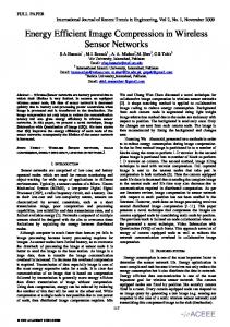
Figure 1. Predicting coding and decoding procedure.
(e.g., [11], [12], [13], [17] [27], [28]) is able to apply to both lossless and lossy data compression scenarios. We believe that an effective unified framework of both lossless and lossy compression is significant and desirable particularly for WSNs, due to the extremely limited resource on tiny motes, as the implementation of two separate lossless and lossy schemes on every mote is clearly not resourceefficient if not impossible. To this end, we present a unified algorithmic framework for both lossless and lossy compression in this paper. Our unified framework is essentially a two-modal Generalized Predictive Coding (GPC), but effectively overcomes the limitations of traditional predictive coding [14, 15], thus enabling an effective and efficient unification of lossless and lossy compression in a systematic manner. Our algorithmic framework is quite simple and its additional complexity compared to the traditional predictive coding is negligible, which makes it well suited for tiny motes in WSN data gathering. Furthermore, we theoretically prove that for lossless compression our proposed framework can perform better than or at least the same as any traditional predictive coding-based schemes regardless of what entropy encoders might be used. We thoroughly evaluate our algorithmic framework in comparison with the recent and effective compression algorithms S-LZW [11], LEC [12] and LTC [13] for real WSN data to illustrate the merits of our approach. Section 2 provides brief backgrounds of traditional predictive coding. Section 3 presents our two-modal transmission framework. In Section 4, our approach is compared with recent temporal compression algorithms including S-LZW and LEC, and LTC using real-world WSN data. Finally, Section 5 gives our conclusions. II.
BACKGROUNDS
Predictive coding was originally introduced by Elias in 1955 [14, 15], based on two breakthrough contributions in the 1940s: Wiener’s work on prediction of random time series [18], and Shannon’s work on the mathematical theory of communication [19]. The communication procedure with predictive coding is illustrated in Fig. 1. Each communication node has a predictor associated with its transmitter, which operates on the past of transmitted messages/signals stored
471
locally to produce an estimate of its future message/signal. An error term (i.e., residue) is calculated by subtracting the predicted message/signal from the actual message/signal. This error term is then used as input to an entropy coder. It is this coded error term that is transmitted to the receiving node. The reversed process is followed at receiving side, with an identical predictor as the sending node. When the error term is received, it is decoded and the original message is then obtained by adding the received error term to the predicted message produced at the receiving node. We can see that predictive coding can be viewed as a two-stage process: (1) message/signal prediction, and (2) error or residue signal coding. In the framework of predictive coding, linear or nonlinear prediction models can be used in the first stage, while a variety of coding schemes are applicable in the second stage, thus providing flexibility for users to select the predictor and entropy encoder for given data sources to better capture the underlying temporal correlations. Wireless sensor networks can be modeled by graphs. A graph G = (V, E), consists of a set of nodes V and a set of edges E V2. Nodes in V represent autonomous communication nodes (e.g., sensor nodes), and edges in E correspond to wireless links among the nodes. Let SINK V denote a small set of particular nodes referred as data sinks where periodically sensed values of physical variables from individual sensor nodes in V should be gathered. The sensor nodes are battery-operated while the sinks are assumed to be not power-limited. A sensor node’s operations beyond medium access control include data transmission, reception, and computation, where transmitting and receiving are the most energy-consuming operations. For example, studies have shown that about 3000 instructions could be executed for the same energy cost as sending a bit for 100 meters by radio [20], in general, receiving has an energy cost that is comparable to that of transmitting. (Note that since the focus of this study is data compression, other energy-efficiency issues associated with MAC layer such as idle listening will not be considered here.) Therefore, it is appropriate and desirable for one to reduce the total energy usage at sensor nodes by carefully minimizing nodes’ transmission (and hence the corresponding reception), offset by a slight increase of computation operations. Predictive coding can fit in such situations where
the high-energy operations of data transmission are minimized at the smaller expense of very low-energy microcontroller’s computation of predictive coding at sensor nodes. For example, a recently proposed lossless entropy compression (LEC) algorithm [12] can be viewed as a specific realization of the predictive coding. The traditional predictive coding paradigm suffers two limitations: (1) no mechanism to (re)synchronize the predictors used at both sensor side and sink side, and (2) potentially bad residue distribution shapes (i.e., “long tails”) in practice having adverse impact on entropy coding performance. In the next section, we introduce our two-modal GPC approach, which can not only overcome these limitations of traditional predictive coding, but also provide an effective and efficient unified framework for both lossless and lossy compression. III.
FRAMEWORK
The basic idea of two-modal generalized predictive coding is to, for a given residue distribution model, encode only those residues falling inside a relatively small range [−R, R] (R > 0 and is called compression radius hereafter) by entropy coding (referred to as predictive compression mode) and to transmit the original raw samples otherwise uncoded (referred to as normal mode). Hence, the two-modal generalized predictive coding is concerned with the adoption of the optimum compression radius Rop to maximize the compression ratio. Clearly, the introduction of normal transmission mode into our framework also provides a direct (re)synchronization mechanism between the predictors at a sensor node and a sink. For WSNs, an atomic sensing information unit in the normal mode of transmission is one raw sensing observation, represented in fixed K bits specified by the precision/resolution of the A/D converter used for sampling. Entropy coding is defined on a set of symbols called an alphabet, or symbol table. The basic alphabet in our framework is defined as follows. The basic alphabet adopted for entropy coding shall contain one symbol S for each residue r to be encoded. Given a compression radius R, one distinct symbol S(i) is used to represent residue r(i) {-R, -R+1, …, 0, …, R-1, R}. The size of the alphabet is 2R+1. It can also be easily seen that given a precision K of A/D converters used in a WSN, the basic alphabet for the traditional predictive coding would then be {-2K+1, -2K +2, …, 0, …, 2K -2, 2K -1}, and the size of the alphabet is 2K+1-1. We hope to work with a very small alphabet for entropy coding in two-modal transmission (needless to say, the size of the basic alphabet in traditional predictive coding is quite prohibitive), to reduce the usage of very limited resource in sensor nodes. A large alphabet would use more memory and would also complicate the computation of compression algorithm. To cope with this issue, the use of an appropriate number system (e.g., decimal system) is adopted in representing individual residues to achieve a reduced alphabet [17]. Another approach is to divide the basic alphabet of residues into groups, such as an Exponential-Golomb type of coding adopted in [12]. In the following sections, we develop our general framework of two-modal generalized predictive coding. In
472
subsection 3.1, we prove that the performance of our framework is superior to that of traditional predictive coding regardless of what entropy encoders are used. In subsection 3.2, we discuss the characterization of sensor noise which can be used to appropriately control and configure lossy compression in WSNs. We finally present our unified lossless and lossy compression framework – two-modal GPC – in subsection 3.3. A. Main Theorem Consider, in a predictive coding framework, a general twosided symmetric residual probabilistic distribution model P(r) centered at zero, where P(r) 0 and P(r) = 1. Let HPC and HGPC denote the entropy of residues of a data source, with the traditional predictive coding framework and the proposed generalized predictive coding framework, respectively. According to Shannon’s information theory, given a probabilistic model of a source, the best that a lossless compression scheme can do is to encode the output of the source with an average number of bits equal to the entropy of the source [21]. We give the following main theorem. Theorem 1: For each residual probability model P(r) with the traditional predictive coding framework, the presented twomodal GPC framework guarantees a bound of an average number of bits that is lower than or equal to that achieved with the traditional predictive coding framework, for any source. That is, HGPC HPC. Proof: Assume that each element in residue sequence is independent. Then, entropy HPC can be expressed as
H PC P( S (i )) log 2 P( S (i )) ,
(1)
where the alphabet S ={S(i)}. The residue entropy HPC provides a lower bound of average bits per symbol for any lossless compression algorithm based on the traditional predictive coding. In the predictive coding framework for sampling precision K, the basic alphabet S ={S(i)} ={-2K+1, -2K +2, …, 0, …, 2K -2, 2K -1}, with total 2K+1-1 symbols. We rewrite (1) as follows:
H PC
P(S (i)) log
P ( S ( i ))1 / 2 K
P ( S ( i ))1 / 2 K
When
P ( S ( i ))1 / 2 K
P ( S ( i ))1 / 2
Thus,
K
2
(2)
P( S (i ))
P( S (i )) 0 , we have
P(S (i)) log
P ( S ( i ))1 / 2 K
P( S (i )) .
P(S (i)) log
2
2
P ( S (i ))
P( S (i )) log 2 (
(3)
1 ), 2K
P(S (i)) log
P ( S ( i ))1 / 2 K
2
P ( S (i )) K
P(S (i)) .
(4)
P ( S ( i ))1 / 2 K
The key point here is that the right hand side of inequality (4) is the average bits transmitted in the normal mode of the two-modal GPC framework with respect to the “optimized” interval [−R, R] for predictive compression mode, as K is the bits of a raw sample, and is the K P ( S (i )) P ( S ( i ))1 / 2
accumulated probability of those raw samples whose resides fall outside of [-R, R]. We immediately obtain the entropy HGPC for the two-modal transmission framework as follows:
P(S (i)) log
H GPC
P ( S ( i ))1 / 2
When
K
P ( S ( i ))1 / 2 K
2
P( S (i )) K
P(S (i)) .
P ( S ( i ))1 / 2
(5)
K
P( S (i )) 0 , one has
P(S (i)) log
2
P ( S (i )) K
P ( S ( i ))1 / 2 K
P(S (i)) 0 .
(6)
P ( S ( i ))1 / 2 K
From (1), (4), (5) and (6), the following holds:
H PC H GPC , H PC H GPC ,
P(S (i)) 0,
P ( S ( i ))1 / 2 K
(7)
otherwise.
Hence, HGPC HPC . This completes the proof. Corollary 1 (Optimum Compression Radius): The optimum compression radius Rop in the two-modal GPC is the smallest R that satisfies the following two conditions: (1) |r| > R P(r) < 1/2K , and (2) |r| R P(r) 1/2K. When there exist more than one R that satisfy the above two conditions, the requirement of the smallest R is to minimize the basic alphabet size for entropy coding in the predictive compression mode. Remarks: The significant implication of this theorem is that the two-modal generalized predictive coding framework indeed provides better lossless compression performance than that of the traditional predictive coding framework, regardless of what concrete entropy encoder is used. The theorem also clearly indicates the condition (see (7)) required on any residual probability models for this performance gain. The corollary explicitly specifies the selection criteria of the optimum compression radius. B. Lossy Compression All kinds of sensors used in sensor networks introduce sensing errors. Typically available only from a sensor’s data sheet provided by its vendor, the only information that can be found describing a sensor’s accuracy is the so-called sensor manufactured error (SME). SME is the maximum margin error that could be produced by a sensor operated normally under given conditions. As larger tolerable compression errors in lossy compression would lead to higher compression ratios, the
473
SME can be used as a base of control knob in lossy compression for data quality. In other words, according to application’s requirements on data quality, the degree of compression errors is bounded and adjustable by a control knob in order to maximize the lossy compression ratio. The idea of our proposed lossy compression is described as follows. When the amount of error (i.e., residue) generated for each sensing sample at a sensor node does not exceed a given margin specified by the control knob, this residue will be approximated as zero in our generalized predictive coding to save more bits. The essence of our approach is based on synchronized iterative multi-step prediction at both sensor nodes and the data sink, in which the predicted output for a given time step will be used as an input for computing the sensing signal series at the next time step, with all other predictor’s inputs being shifted back one time unit. This is in contrast with the lossless compression in generalized or traditional predictive coding where the single-step prediction is used at both sensor nodes and the sink. As prediction errors propagate in this iterative multi-step prediction procedure, eventually a residue would become larger than the allowed error bound. At this point, the compression mode has to be switched to the normal mode in our GPC, and the original raw reading(s) will be transmitted. The number of raw readings to be transmitted is equal to the input dimension of predictor used for the sake of resynchronization of predictors at both the sensor node and the sink. We can see now that the embedded normal mode for transmitting raw samples in our generalized predictive coding framework has been able to directly support an iterative multi-step prediction scheme to facilitate lossy compression. That is, in addition to the performance improvement on lossless compression over the traditional predictive coding framework, as shown by the main theorem in the previous subsection. The unification of both lossless and lossy compression in the presented generalized predictive coding framework is significant, as meaningful lossy compression is difficult to achieve in the traditional predictive coding framework, unless some complex lossy encoder is employed. C. Unified Algorithmic Framework Our proposed generalized predictive coding is a unified algorithmic framework of both lossless and lossy compression. In our unified algorithmic framework, a compression error bound (denoted as e) can be used as the control knob, where lossless compression can be processed as e=0 in our framework. The algorithmic procedure at source nodes of the GPC is presented in Figure 2. The corresponding algorithmic procedure at the sink(s) can be described accordingly. Note that the proposed GPC is a general framework in which one has complete flexibility to choose an appropriate predictor and entropy encoder based on given tasks. IV.
SIMULATIONS AND ANALYSIS
To thoroughly evaluate the proposed generalized predictive coding framework, we first compare its lossless compression performance with LEC algorithm and S-LZW algorithm using real-world WSN datasets from SensorScope [22]. Since LEC and S-LZW represent two different approaches in lossless
Notation: e: given compression error bound; x: sensor reading; prediction of x; xˆ : residue: x xˆ ; R: compression radius (e R); predictor(): any predictor used to predict the next observation based on the previous observations or predictions; p: the input demission of predictor; flag: the flag to indicate the predictor (re)synchronization status; lossy: the flag indicate if information loss occurred; encode(): encode residues with any encoder being used; pack(y, n): packing n data items y at source node to into a packet; send(): transmitting at source node. GPC (e): begin flag TO_SYNC; while (not_done) if (flag = TO_SYNC) then pack (x, p); flag SYNC_DONE; lossy 0; else xˆ predictor(); residue x xˆ ; if (e = 0) then /* lossless compression */ if (residue R) then pack(encode(residue), 1); else pack(x, 1); if (e 0) then /* lossy compression */ if (residue 0 and residue e) then pack(encode(0), 1); lossy 1; else if (residue e and residue R) then pack(encode(residue), 1); else if (lossy =0) then pack(x, 1); esle flag TO_SYNC; send(); end Figure 2. Two-modal generalized predictive coding framework.
compression for WSN data as briefly described in Section 1, they form a good set of existing algorithms for our lossless compression evaluation. We then evaluate our framework’s lossy compression performance by comparing it with the performance of the representative LTC algorithm using the same real-world WSN datasets. The compression performance is usually evaluated by compression ratio defined as follows:
s' s' CR (1 ) 100% (1 ) 100% KN s , where s and s’ denote the original raw data size and the compressed data size in bits, respectively; N is the number of total data samples, and K is the fixed bits per raw sample specified by the precision of the A/D converter used for sampling.
474
TABLE I. CODING TABLE USED IN THE SIMULATIONS FOR THE PROPOSED TWO-MODALGENERALIZED PREDICTIVE CODING FRAMEWORK WITH K=14 ni 0 1 2 3 4 5 6 7 8 9 10 11 12 13 14
si 00 010 011 100 101 110 1110 11110 111110 1111110 11111110 111111110 1111111110 11111111110 111111111110
ri (ni {0,1,…,13}) / Original raw sample (ni =14) 0 -1,+1 -3, -2,+2,+3 -7, … , -4, +4, …, +7 -15, … , -8, +8, …, +15 -31, … , -16, +16, …, +31 -63, … , -32, +32, …, +63 -127, … , -64, +64, …, +127 -255, … , -128, +128, …, +255 -511, … , -256, +256, …, +511 -1023, … , -512, +512, …, +1023 -2047, … , -1024, +1024, …, +2047 -4095, … , -2048, +2048, …, +4095 -8191, … , -4096, +4096, …, +8191 Original raw sample
LEC employs the popular and simple differentiation predictor to predict the next sample based on the last observed sample, that is, xˆi xi 1 . Then, the residue is the difference ri xi xi 1 . The entropy encoder in LEC is a modified version of the Exponential-Golomb code of order 0 [23]. To make the comparisons between our framework and the published algorithms (e.g., LEC and S-LZW) fair and straightforward, we adopted the identical predictor, residual distribution model and entropy encoder employed in LEC [12] in the experiments of our two-modal GPC framework’s predictive compression mode. Based on the residual model adopted, the compression radius R is simply selected as 2K-1-1. In the normal mode of the two-modal GPC, uncompressed raw samples are transmitted, following the same assumption of byte-aligned representation of uncompressed raw samples in [12]. Thus, the coding table employed in our two-modal GPC framework in the simulations is given in Table 1. Our coding table (i.e., 15 entries) has the same size as that of the coding table used in LEC [12], whereas S-LZW uses significantly more memory space for its dictionary entries and mini-cache entries (e.g., MAX_DICT_ENTRIES being 512, and MINICACHE_ENRTIES being 32, [12], [11]). A. Data Sets Real-world, publically accessible environmental monitoring WSN datasets from SensorScope are used in our simulations [22]. To compare with the recently proposed algorithms LEC and S-LZW, the same temperature and relative humidity measurements from the identical sensor nodes used in [12] in the following four SensorScope deployments are tested: HES-SO FishNet, LUCE, Grand-St-Bernard, and Le Génépi. A Sensirion SHT75 sensor module [24] was adopted with TinyNode sensor node platform [25] in the SensorScope deployments. Both the temperature and relative humidity sensors are connected to a 14-bit ADC. However, the outputs of ADC for the raw temperature (raw_t) and raw relative humidity (raw_h) are represented with resolutions of 14 and 12 bits, respectively. These raw outputs raw_t and raw_h are then converted into physical measures t and h expressed, respectively, in Celsius degrees and percentage (%) as described in [24]. The data sets published on SensorScope corresponding to the four deployments are in the format of physical measures t and h. Therefore, one needs to convert such physical measures back to their corresponding raw measures to evaluate compression algorithms, which can be realized by using the inverted versions of the conversion functions in [24]. For more details about characteristics of these data sets, please see [12]. B. Lossless Compression Results The lossless compression performance of the two-modal GPC together with the other lossless compression algorithms LEC and S-LZW is listed in Table 2 for the temperature and relative humidity data sets from the four WSN deployment sites (the compression ratios by S-LZW adopted from [12]). The compression ratios obtained by our two-modal GPC framework are almost identical to those obtained by LEC, and are significantly better than those of S-LZW. Also, the GPC’s lossless compression complexity is essentially the same as that
475
TABLE II.
LOSSLESS COMPRESSION PERFORMANCE COMPARISONS Compression ratio CR (%)
Variable
Temperature
Relative humidity
Data set FN_ID101 LU_ID84 GSB_ID10 LG_ID20 FN_ID101 LU_ID84 GSB_ID10 LG_ID20
Two-modal GPC 64.34 70.52 58.38 54.05 60.79 61.95 52.68 48.82
LEC
S-LZW
64.46 70.61 58.48 54.13 60.94 62.07 52.83 49.00
30.35 48.99 26.86 22.02 36.27 31.24 24.92 21.93
of LEC [12], and thus is less than 1/6 and 1/17 of the S-LZW complexity for temperature and relative humidity data, respectively [12] (see Table 11 of [12]). We provide the following insight into the performance comparison results between the two-modal GPC and the LEC. First, all eight WSN data sets selected in [12] have quite smooth environmental data, for which the differentiation predictor can generate a very good shape of residue distributions. It turns out that the two-modal GPC essentially produces a compression ratio equal to that of LEC for those selected data sets, because HPC = HGPC for these data sets. A question arises here: why do the given results show that the two-modal GPC’s compression ratios were slightly lower than those of LEC’s? This can be explained by the LEC’s hidden constraint/requirement on the handling of the transmission of its first sample of a block. LEC, like any other compression algorithm based on a traditional predictive coding framework, suffers from the problem of lacking a mechanism for predictor’s resynchronization. One issue here is how the first p samples (p being the order of the predictor used) are received at the sink first in order to restore the rest of original samples from the encoded residues. LEC’s solution relies on an enforced hidden rule that the first p “residues” of a block of given size (i.e., 512 bytes used in [12]) are actually original samples, not residues. A fundamental drawback of this hidden rule is the assumption of no any packet loss in communications, because each packet cannot be decompressed at the sink without the packets that proceed it in a same block. We note that the compression performance of LEC shown in Table 2 is subject to this hidden rule. In contrast, our framework is free of this hidden rule due to its normal transmission mode, providing a complete flexibility for compressing and decompressing each individual packet in a block independently. Given the nature of unreliable communication channels of WSNs, our GPC is significantly more robust than LEC. C. Lossy Compression Results In lossy compression, the control knob of compression error bound e can be conveniently specified as a percentage of sensor manufactured error SME. For example, if e = 100% of SME, the possible maximum compression error for each individual raw sample is bounded by the degree of SME. We conduct experiments on lossy compression using the twomodal GPC for different values of compression error bound e. The compression ratios for temperature and relative humidity
data sets achieved by the two-modal GPC with different values of e are shown in Figures 3 and 4, respectively. Note that in Figures 3 and 4, e = 0 indicates lossless compression. One interesting observation is that when e (e>0) is small, the compression performance actually degraded compared to that of the lossless compression (e.g., e=0) in the two-modal GPC. At first glance, this appears to contradict intuition. In fact, when e is small, it is possible that the gain obtained from approximating small residues as zeros in lossy compression may not be sufficient to overcome the overhead involved in frequent predictor resynchronizations via the normal transmission mode in which raw samples instead of residues have to be transmitted. As e becomes larger, the compression ratio will eventually be significantly higher than that of lossless compression, even when the e only reaches 100% of SME.
Next, we compare the lossy compression performance of the two-modal GPC with that of LTC. Figures 7 and 8 (see next page) show the LTC’s compression ratios over compression error bound e for temperature and relative humidity data sets respectively for the four sensor nodes. Due to the underlying nature of piecewise linear approximation for LTC, it can be observed that LTC would produce negative CR if it were used for lossless compression (i.e., e=0), indicating that the size of the lossless-compressed data is actually larger than the original sampling data. This reflects the fact that lossless and lossy compression schemes typically are based on different underlying principles.
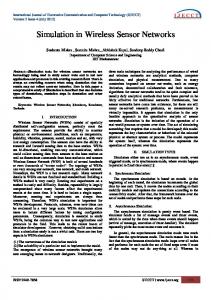
To give a feeling of lossy compression, Figures 5 and 6 show the comparison between the original and the reconstructed data samples of the FN_ID101, GSB_ID10, LG_ID20, and LU_ID84, for temperature and relative humidity data sets, respectively, performed by the two-modal GPC.
Figure 5. Comparison between the original and the reconstructed temperature data samples of the FN_ID101, GSB_ID10, LG_ID20, and LU_ID84, performed by the two-modal GPC with e = 60% of SME.
Figure 3. Compression ratio CR vs. compression error bound e obtained by the two-modal GPC for WSN temperature data sets, where e is from 0 to 200% of SME.
Figure 6. Comparison between the original and the reconstructed relative humidity data samples of the FN_ID101, GSB_ID10, LG_ID20, and LU_ID84, performed by the two-modal GPC with e = 100% of SME. Figure 4. Compression ratio CR vs. error bound e by the two-modal GPC for WSN relative humidity data sets, where e is from 0 to 200% of SME.
476
By comparing compression ratios shown in Figures 3 and 4 to those shown in Figures 7 and 8, we can see that LTC outperforms the two-modal GPC framework only when the compression error bound becomes sufficiently large, and the error bound threshold varies from data set to data set. We also observe that the lossy compression ratio of the two-modal GPC increases more modestly than that of LTC as the tolerable compression error bound increases.
and lossy compression for WSNs. Performance comparisons between our two-modal GPC and recently proposed effective lossless compression algorithms LEC and S-LZW as well as lossy compression algorithm LTC using real-world WSN data sets are reported and analyzed. Using the same real WSN data sets adopted in [12], we show that the two-modal GPC significantly outperforms S-LZW, and has the same performance as that of LEC but completely fixing LEC’s “problem of the first sample” [12]. In general, the two-modal GPC completely overcomes the predictor (re)synchronization problem suffered by any other lossless compression algorithms based on traditional predictive coding, including the problem of the first p samples (p being the order of the predictor used). The evaluation of the two-modal GPC with LTC for lossy compression shows that two-modal GPC’s compression performance is generally better than that of LTC when the error bound is small, but slightly worse than that of LTC when the error bound becomes large. Based on the proposed twomodal GPC framework, we have designed and implemented a compressed data-stream protocol (CDP) for bulk data collections in WSNs [30]. Our on-going work includes further testing and evaluating our two-modal GPC framework and CDP protocol in a real-world WSN testbed deployed for environment monitoring.
Figure 7. Compression ratio CR vs. error bound e obtained by the LTC for WSN temperature data sets, where e is from 0 to 200% of SME.
ACKNOWLEDGMENT This work is supported by National Science Foundation under grant CNS-0758372. Simulations were conducted by graduate students W. Peng and Y. Li. REFERENCES [1]
Figure 8. Compression ratio CR vs. error bound e by the LTC for WSN relative humidity data sets, where e is from 0 to 200% of SME.
V.
CONCLUSIONS
In this paper, we extend and generalize traditional predictive coding, and develop a unified algorithmic framework referred to as two-modal generalized predictive coding for both lossless and lossy compression. We give analytical proof to show that the proposed two-modal generalized predictive coding framework achieves optimal lossless compression performance in comparison to traditional predictive coding framework. This proposed unified framework is simple and efficient, and is particularly suited for highly resource-constrained WSN nodes where both lossless and lossy compressions are needed in applications. To our knowledge, this is the first work on the unification of lossless
477
C. Intanagonwiwat, R. Govindan, and D. Estrin, “Directed diffusion: A scalable and robust communication paradigm for sensor networks,” Proceedings of IEEE MobiCom, Aug. 2000. [2] W. Heinzelman, A. Chandrakasan, and H. Balakrishnan, “EnergyEfficient Communication Protocol for Wirelesss Mircrosensor Networks,” International Conference on System Sciences, 2000. [3] C. Pandana and K. J. R. Liu, “Near-Optimal Reinforcement Learning Framework for Energy-Aware Sensor Communications,” IEEE Journal on Selected Areas in Communications, vol. 23, pp. 788-797, April 2005. [4] T. van Dam, and K. Langendoen, “An Adaptive Energy-Efficient MAC Protocol for Wireless Sensor Networks,” Proceedings of 1st Int’l Conf. on Embedded Networked Sensor Systems, 2003. [5] W. Ye, J, Heidemann, and D. Estrin, “Medium Access Control with Coordinated Adaptive Sleeping for Wireless Sensor Networks,” IEEE/ACM Transactions on Networking, vol. 12, pp. 493-506, 2004. [6] S. Bandyopadhyay and E. J. Coyle, “Spatio-Temporal Sampling Rates and Energy Efficiency in Wireless Sensor Networks,” Proceedings IEEE INFOCOM, vol. 3, pp. 1728-1739, 2004. [7] S. Bandyopadhyay, Q. Tian, and E. J. Coyle, “Spatio-Temporal Sampling Rates and Energy Efficiency in Wireless Sensor Networks,” IEEE/ACM Transaction on Networking, vol. 13, pp.1339-1352, 2005. [8] A.D. Marbini and L.E. Sacks, “Adaptive Sampling Mechanisms in Sensor Networks,” London Communications Symposium, UK, 2003. [9] G. Anastasia, M. Contib, M. D. Francescoa, and A. Passarella, “Energy conservation in wireless sensor networks: A survey,” Ad Hoc Networks, Vol. 7, No. 3, pp. 537-568, 2009. [10] E. Fasolo, M. Rossi, J. Widmer, and M. Zorzi, “In-network Aggregation Techniques for Wireless Sensor Networks: A Survey,” IEEE Wireless Communications, Vol. 14, pp. 70-87, 2007. [11] C.M. Sadler, and M. Martonosi, “Data Compression Algorithms for Energy-Constrained Devices in Delay Tolerant Networks,” Proc. 4th
[12]
[13]
[14] [15] [16] [17]
[18] [19] [20]
ACM Int. Conf. Embedded Networked Sensor Systems, Boulder, Colorado, USA, October 31–November 3, pp. 265–278. ACM, New York, NY, USA, 2006. F. Marcelloni and M. Vecchio, “An Efficient Lossless Compression Algorithm for Tiny Nodes of Monitoring Wireless Sensor Networks,” The Comp. J., vol. 52, pp. 969-987, 2009. T. Schoellhammer, E. Osterweil, B. Greenstein, M. Wimbrow, and D. Estrin, “Lightweight Temporal Compression of Microclimate Datasets,” Proc. 29th Annual IEEE Int. Conf. Local Computer Networks, Tampa, FL, USA, November 16–18, pp. 516–524, 2004. P. Elias, “Predictive coding I,” IRE Trans. Information Theory, vol. 1, no.1, pp. 16–24, Mar. 1955. P. Elias, “Predictive coding II,” IRE Trans. Information Theory, vol. 1, no.1, pp. 24–33, Mar. 1955. T. A. Welch, “A Technique for High-Performance Data Compression,” IEEE Computer, vol. 17, pp.8–19, June 1984. C. Liu, K. We, and J. Pei, “An energy-efficient data collection framework for wireless sensor networks by exploring spatiotemporal correlation,” IEEE Trans. Parallel and Distributed Sys., vol. 18, no. 7, pp. 1010-1023, July 2007. N. Wiener, Extrapolation, Interpolation, and Smoothing of Stationary Time Series, Cambridge, MA: MIT Press, 1949. C. E. Shannon, “A mathematical theory of communication,” Bell Syst. Tech. J., vol. 27, pp.379–423, pp.623–656, 1948. J. Pottie, W. J. Kaiser, “Embedding the internet wireless integrated network sensors,” Communications of the ACM, vol. 43, no. 5, pp. 51– 58, May 2000.
478
[21] K. Sayood, Introduction to Data Compression (3rd ed), Morgan Kaufmann Publishers, US, 2006. [22] SensorScope deployments homepage http://sensorscope.epfl.ch/index.php/Main_Page (accessed 2011). [23] J. Teuhola, “A compression method for clustered bit-vectors,” Inf. Process. Lett., vol.7, pp. 308–311, 1978. [24] Sensirion homepage (2009) www.sensirion.com (accessed 2011). [25] TinyNode homepage (2009) http://www.tinynode.com (accessed 2011). [26] A, Kiely, M. Xu, W.-Z. Song, R. Huang, and B. Shirazi, “Adaptive Linear Filtering Compression on Realtime Sensor Networks,” Proceedings of IEEE International Conference on Pervasive Computing and Communications, pp. 1-10, 2009. [27] S. Goel and T. Imielinski, “Prediction-based monitoring in sensor networks: taking lessons from MPEG,” SIGCOMM Comput. Commun., vol. 31, pp. 82-98, 2001. [28] N. D. Pham, T. D. Le, and H. Choo, “Enhance exploring temporal correlation for data collection in WSNs,” IEEE International Conference on Research, Innovation and Vision for the Future, pp.204-208, 2008. [29] C. T. Chou, R. Rana, and W. Hu, “Energy efficient information collection in wireless sensor networks using adaptive compressive sensing,” IEEE 34th Conference on Local Computer Networks, Zürich, Switzerland, 2009. [30] N. Erratt, and Y. Liang, “CDP: A Compressed Data-Stream Protocol for Wireless Sensor Networks,” submitted.