2 The MathWorks, Inc., Application Engineering, 39555 Orchard Hill Place, Novi, ... 3 The MathWorks, Inc., xPC Target Development, 3 Apple Hill Dr., Natick, MA.
Embedded Real-Time Control via MATLAB, Simulink, and xPC Target Pieter J. Mosterman1 , Sameer Prabhu2 , Andrew Dowd3 , John Glass1 , Tom Erkkinen4 , John Kluza5 , and Rohit Shenoy6 1
2
3
4
5
6
The MathWorks, Inc., Simulink Development, 3 Apple Hill Dr., Natick, MA 01760-2098, U.S.A. The MathWorks, Inc., Application Engineering, 39555 Orchard Hill Place, Novi, MI 48375-5374, U.S.A. The MathWorks, Inc., xPC Target Development, 3 Apple Hill Dr., Natick, MA 01760-2098, U.S.A. The MathWorks, Inc., Technical Marketing, 39555 Orchard Hill Place, Novi, MI 48375-5374, U.S.A. The MathWorks, Inc., Application Engineering, 3 Apple Hill Dr., Natick, MA 01760-2098, U.S.A. The MathWorks, Inc., Technical Marketing, 3 Apple Hill Dr., Natick, MA 01760-2098, U.S.A.
1 Introduction This article shows how xPC Target [44] facilitates embedded control system design by turning general-purpose personal computer (PC) hardware into a rapid prototyping platform. The PC-based platform used is the MathWorks TM R [31], xPC TargetBox [45], an industrial PC. xPC Target is integrated in Simulink enabling the use of Simulink as a graphical front-end with MathWorks tools for parameter estimation, response optimization, and linearization throughout the design cycle. 1.1 What is an embedded control system? A control system is an implemented strategy used to cause a physical system, or plant, to behave in a desired manner. There are two types of control strategies: • •
Closed-loop control uses feedback measurements to correct error between the plant output and a reference input, i.e., the desired behavior. Reactive control is event driven and interacts with the plant via state transition behavior.
As the feedback control strategy increases in complexity, it becomes more difficult to apply analog components for its implementation. Dynamics in
2
P. J. Mosterman et al.
an analog feedback control loop always interact, making it more difficult to match desired controller characteristics. For example, an analog system always has a limited filter quality factor, Q, due to parasitic impedances and other limitations. Conversely, it is easy to create an extremely sharp digital filter with very large Q. Another complication is that analog integrators are always limited by capacitor leakage, yet digital integrators can be nearly perfect. A processor-based approach usually works best for reactive control as well. In modern control systems, the control strategy is thus typically implemented in software. A microprocessor determines the input to manipulate the plant and this requires facilities to apply this input to the physical world. In addition, the control strategy typically relies on measured values of the plant behavior that have to be made available to the computing resources. The immersion of computing power into the physical world is one characteristic of an embedded control system. The other characteristic is that the software that implements the control strategy is stored in read-only memory. Thus, unlike a general-purpose computer, an embedded control system is not independently programmable. In other words, an embedded control system is expected to function without user intervention, although it may require user interaction. 1.2 Embedded control system characteristics The general configuration of an embedded control system is shown in Fig. 1. Because the controller operates in the low-power electronics domain and the plant operates in high-power hydraulics, mechanics, thermal, and other physical domains, transducers are needed to convert between controller and plant. These transducers are used either by actuators, to drive the plant with controller-computed values, or by sensors, to provide measurements to the low-power electronics domain. In embedded systems, the low-power computational electronics of the controller has to interact with high-power physical domains of many types [42].
Fig. 1. General embedded control system configuration
For example, consider the Stewart platform in Fig. 2. This physical system consists of six legs supporting a circular platform. The platform may be used
Embedded Real-Time Control via MATLAB, Simulink, and xPC Target
3
to build, for example, an aircraft simulator. The legs are then used to move the simulated aircraft so as to give the impression of being inside an actual aircraft. This unit is sometimes called a “hexapod,” after its six legs.
Fig. 2. A Stewart platform
To move the platform, each leg is equipped with a motor that extends it. The control strategy that computes the desired extension is implemented in a low-power microprocessor. An amplifier turns this electrical signal into a high-power equivalent that can be used to drive the motor. Sensors measure the actual extension of the legs. Six linear encoders, one on each leg, send a voltage pulse every time the leg slides a given distance. Dedicated counter hardware counts the number of pulses. The actual distance is computed based on this count. In addition to the transformation between high- and low-power domains, transformations between discrete-time and continuous-time behavior are required. The plant can be viewed as changing continuously in time [14, 27]. The controller, however, has a discrete clock that governs its behavior, and so its values change only at discrete points in time. To obtain deterministic behavior and ensure data integrity, the sensors must include a mechanism to sample continuous data at discrete points in time, while the actuators need to produce a continuous value between the time points with discrete-time data (typically, the value is held constant). 1.3 Rapid prototyping in embedded control system design Formal control design methods invariably rely on a plant model [1, 4]. The plant model can be derived from first principles but often contains unknown parameters. Experiments must be conducted to gather information on the behavior of the plant dynamics to help estimate these parameters.
4
P. J. Mosterman et al.
Once a plant model is available, closed-loop feedback and reactive control can be designed using simulation or synthesized using methods such as pole placement, inverse dynamics, total energy control, H∞ , and model predictive control. Rapid prototyping tools support this design paradigm. At the start of the control design process an engineer may have an inaccurate model or no model at all. At this stage, a skeleton control system is developed to stabilize a system and to obtain the desired behavior for the experiment. Experiments can then be designed and performed to acquire responses of the system under various operating conditions. The acquired data can then be used to enhance the plant model and to design a new control system based on the more accurate plant model. Simulating the combined control system and plant model, the designer can study and optimize the performance of the system using the full nonlinear plant simulation model. Finally, the control system can be implemented on a rapid prototyping system. If the system does not meet the performance achieved in simulation, the model and the control system design are further refined. Such incremental design for embedded control systems requires that the rapid prototype operate in real time, interact with hardware, have supporting control functionality, and be safe. 1.4 Chapter overview In Section 2, the concept of rapid prototyping is elaborated. In Section 3, the Stewart platform is presented that will be used throughout the chapter to illustrate the concepts put forward. Section 4 discusses the PC-based xPC Target for rapid prototyping, and Section 5 describes the industrial xPC TargetBox that is used to implement the embedded control for the Stewart platform. In Section 6, generation of the embedded code for control is discussed. Section 7 discusses how models are obtained. Section 8 explains how to acquire the data necessary for modeling. Section 9 gives an overview of how models are used in the embedded control system design. Section 10 describes the control strategy as used for the Stewart platform, and Section 11 presents conclusions.
2 What Is Rapid Prototyping? Much research has been devoted to the analysis, design, and synthesis of a controller based on a plant model. Note that this research pertains to a model of the controller as well. Once this controller model has been designed, however, it still has to be realized and connected to the actual plant, and most of the actual control system engineering effort is devoted to taking the controller model to such a realization. In particular, accounting for some of the implementation details such as, for example, the resolution of a fixed-point
Embedded Real-Time Control via MATLAB, Simulink, and xPC Target
5
microprocessor that will be used, may affect the originally designed controller model and require it to be modified [20]. A rapid prototype is a quick way to validate the controller code by executing it with the actual plant, sensors and actuators, the plant model, or any combination of these components [19]. The purpose of rapid prototyping is to obtain confidence and pinpoint flaws and errors in a partial design before committing to a completed design. This is a common design approach. For example, in software, a core algorithm is typically implemented and tested before extensive comments, exception handling, and robustness functionality are added. In scientific research and education, where a system is rarely taken into production, rapid prototyping serves an important purpose. In industry, rapid prototyping allows testing of a partial design before expending the effort to include robustness measures and optimizing the design. There are three different rapid prototyping configurations: functional, bypass, and on-target (Fig. 3). •
•
•
Functional rapid prototyping is used for testing new ideas and research projects where there is no controller or the controller is too primitive to support advanced control strategies. In such cases, the rapid prototyping controller controls the entire system. As the focus is on proving the concept, the size of the generated code and the fixed-point characteristics of the software are not important. The hardware used for functional rapid prototyping is often PC-type hardware and is not intended for production controller applications. The flexibility to add I/O hardware is important in rapid prototyping as various hardware contingencies cannot be accounted for ahead of time. Bypass rapid prototyping replaces only a part of the existing control system with the new controller. This is useful if the system control demands high current capacity drivers that are typically not available in rapid prototyping controllers or if only part of the functionality of the controller needs to be replaced with the new features. On-target rapid prototyping uses the production hardware directly and captures all the hardware dependencies and I/O limitations [5, 12]. It allows engineers to assess the ability of the algorithm to control a vehicle under various test track conditions, especially those, such as ice, that are hard to simulate using a model.
3 A Stewart Platform This example describes the rapid prototyping of the Stewart platform shown in Fig. 2, using xPC Target [44] and xPC TargetBox [45].
6
P. J. Mosterman et al.
Host
Target
Modeling and Simulation
Real-Time Application
MS Windows
Real-Time Kernel
PC Non Real-Time
PC Real-Time
Functional
Bypass
On-Target
Fig. 3. Rapid prototyping configurations.
3.1 Control objectives One control objective is to enable the Stewart platform to assume a prescribed position as accurately and quickly as possible. Another is to move the platform at specific speeds. 3.2 System configuration The Stewart platform system in Fig. 4 shows the hexapod plant and xPC TargetBox controller connected by sensors and actuators. xPC TargetBox includes a 400 MHz Intel Pentium III (floating-point) processor, with 128 MB RAM, and 32 MB flash RAM. 3.3 The peripherals The peripheral hardware consists of force actuators and position sensors. Force actuators Mounted on the legs of the Stewart platform are Nanomotion H1 piezoceramic motors that extend the legs, so there are six actuators. The motors are driven by Nanomotion amplifiers that read the control voltage from one of the six channels of the RTD DM6604 analog output of the xPC TargetBox. The input to the amplifiers is a low-power analog reference signal that they convert into a high-power sinusoidal voltage. By varying the amplitude of the sinusoid, the motor moves the leg up and down.7 7
http://www.nanomotion.com/data/docs/Tech%20notes%20102.pdf
Embedded Real-Time Control via MATLAB, Simulink, and xPC Target
7
9 pin D connector 2 x 40 kHz sine wave with Nanomotion Nanomotion varying amplitude piezo motor amplifier
hexapod
0/+5 [V] grated glass slide electrical and MicroE systems pulses encoder pickup
9 pin D connector
RTD DM 6814 RTD DM 6604 D/A +10/-10 [V] motor velocity command signal (limited in software to +7/-7 [V])
programmable FLASH
Incremental encoder board reads encoder counts on 6 channels
xPC Targetbox TCP/IP - TCP/IP to download and control the target model - UDP to send command signal from the space mouse and predefined trajectory
USB x,y,z, roll,pitch,yaw host PC
space mouse
Fig. 4. Stewart platform hardware configuration
Position sensors Six MicroE Mercury 3110 incremental encoders8 measure the extension of each of the six legs. To measure the extension, these sensors use an optical beam that produces a sequence of electrical pulses when a grated slider is passed by. The slider has 65,536 counts on it over about 4 cm of travel, giving a precision of about 0.61 µm of travel per count. A slide with a reference marking calibrates the zero location from which to start counting incrementally. In this particular hardware setup, the encoder pickups cannot see the reference marking and so have a purely incremental capability. Because the encoder cannot be reset at a given location based on a reference reset pulse, the only option is to drive it to the stops of the actuator slider and define that to be zero. The sensor is powered by a 5 V supply at 300 mA. It delivers the electrical pulses with a power and impedance that allow it to be directly connected to a counter board. xPC TargetBox includes an RTD DM6814 incremental encoder board that counts how many pulses it receives from the encoder pickup and passes this count to the model. Two counter I/O boards, each supporting three channels, are used.
4 xPC Target 4.1 General-purpose hardware A rapid prototyping platform needs to be more powerful and flexible than the eventual target processor. For example, if the software has not yet been 8
http://www.microesys.com/
8
P. J. Mosterman et al.
optimized, it will not run as efficiently. To achieve real-time behavior, a more powerful microprocessor is necessary. Furthermore, additional measurements may need to be made to obtain insight in the functioning of the controller. The necessary flexibility, computing power, and memory capacity may make rapid prototyping platforms much more expensive than the hardware that is ultimately used in production. Because of the cost, rapid prototyping platforms are often used for more than one project, an approach that is supported by the inherent flexible nature of such platforms. xPC Target [44] provides the means to turn general-purpose PC hardware into a prototyping environment that can be used for signal acquisition, rapid prototyping, and hardware-in-the-loop simulation. 4.2 PC form factor The form factor of a device is its physical shape and size. There are a number of specific form factors available for PC-based systems. A form factor may encompass design components such as connector types, bus protocols, board sizes, power specifications, and mechanical enclosures. Rarely does the form factor directly influence processor selection, but a particular form factor is often indirectly tied to a processor family. Thus, it is common to couple the choice of a form factor to the processor selected. This can be a regular desktop PC, rack-mounted PC, or an industrial PC. The advantages of using PC-based platforms are their scalable computing power, flexibility, and expandability. R R xPC Target can be used with any PC containing Intel 386/486, Pentium , or AMD K5/K6/Athlon processors as the real-time target. This includes desktop computers, industrial computers such as xPC TargetBox, PC/104, PC/104+, CompactPCI, all-in-one embedded PC, or any other PC-compatible form factor. Thanks to economies of scale and competition, these devices have performances in the order of millions of floating-point operations per second (MFLOPS), relative to cost. Moreover, the large range of available form factors allows xPC Target to be used in small PC/104 systems as well as in much larger expanded PCI systems. For example, it is common to perform early design work using a standard desktop PC and then immediately retarget the control algorithm to an industrial computer for field testing. 4.3 Real-time operating system The xPC Target kernel provides a real-time operating system that supports both interrupt handling and polling and is tuned to provide maximum performance with minimal overhead. High-performance hardware allows sample rates that approach 100 kHz. 4.4 Drivers A key step in transforming software into a real-time system is the requirement to have device drivers that communicate between the I/O devices on the target
Embedded Real-Time Control via MATLAB, Simulink, and xPC Target
9
PC and the application code running on this target. These drivers thus enable interaction between the real-time application and the real physical system. The device driver contains the code that runs on the target hardware for interfacing to I/O devices such as analog-to-digital (A/D) converters, encoders, digital signals, and communication ports. Each device driver is implemented as a Simulink S-function using C-code MEX files. Figure 5 shows the Simulink blocks for the six encoder channels supported by two DM6814 boards used on the Stewart platform. These blocks result in automatically generated code for the hardware drivers.
6
voltage
position
motors
DM6604 act_extend 6
hexapod
grated_slides
6
DM6814
6
voltage des_extend
6 postion
controller 6
3
position
position
3
positions
translation
3
Translation
leg_extend angle
convert_to_legs_extension
3
angle
UDP_from_host
angle
UDP_to_target
3
angles
rotation
3
limit_and_filter 12
Rotation
Buttons
Magellan Space Mouse
Fig. 5. Simulink model of Stewart platform host and target software
The code for the entire system identification application can be generated without manually producing glue or driver software. 4.5 Writing device drivers To understand the process of writing device drivers, it is essential to understand S-functions and low-level programming of I/O boards. An S-function is a description of a Simulink block written in a language such as M or C [31]. S-functions have a special calling syntax, referred to as a call-back, that allows these custom blocks to interact with Simulink in the same manner as built-in Simulink blocks do. A C S-function can be compiled and dynamically linked into the Simulink environment, thereby allowing custom blocks to be added to the Simulink environment. Thus, S-functions and S-function routines form an application program interface (API) that allows the flexible implementation of generic algorithms within the Simulink environment. This flexibility cannot always be maintained when S-functions are R [28] to generate code. For example, it is not used with Real-Time Workshop R [18] workspace from an S-function that is possible to access the MATLAB used with Real-Time Workshop, but it is possible when using the S-function with Simulink for simulation purposes only.
10
P. J. Mosterman et al.
To incorporate a device driver block in the Simulink model requires an Sfunction, which in turn requires the C source code for the device driver. xPC Target provides a comprehensive device driver library supporting more than 250 boards of various types, including A/D converters, digital input/output, Controller Area Network (CAN) [3], and ARINC 429. Thus, xPC Target greatly simplifies the process of generating a real-time application by providing the library of device driver S-functions. Writing a device driver that is not yet available is simpler for xPC Target than writing a general configuration since xPC Target does not contain the many layers typically found in an operating system (OS). For example, the xPC Target kernel has direct virtual-to-physical address mapping, which means that declaring a pointer at a particular address will lead to bus access at the same physical address. Moreover, the source code for the existing xPC Target device drivers is provided with the product, enabling users to gain familiarity with the way device drivers are implemented. Device drivers for xPC Target can be developed in one of two ways: • •
Obtaining the source code for the driver from the hardware manufacturer and porting it to the xPC Target kernel Using the register programming manual of the I/O board from the hardware manufacturer to develop a driver from the very beginning
The xPC Target kernel provides a set of functions for accessing ports and memory, PCI initialization space, and performing time measurements that can be used in an S-function compiled for xPC Target. PCI boards are better than ISA boards for adding I/O functionality to a real-time system because they provide plug-and-play allocation of access, interrupt resources, a wider and faster bus, and software calibration. 4.6 xPC Target configuration The xPC Target host-target arrangement is shown schematically in Fig. 6. On the host PC (which runs MATLAB, Simulink, Real-Time Workshop, and xPC Target), xPC Target works with the code generated from the Simulink application and a C compiler to build the real-time target application. The target application can run in real time on a target PC once it is downloaded to the target PC from the host PC. The target hardware is booted from a real-time kernel in xPC Target. However, the xPC Target kernel needs the PC basic input/output system (BIOS) because when the target PC boots and the BIOS is loaded, the BIOS prepares the target PC environment for running the kernel and then starts the kernel. The kernel initiates the host-target communication, activates the application loader, and waits for the target application to be downloaded from the host PC. The host-target communication can occur through either serial or TCP/IP communication protocols. Once the target application has been
Embedded Real-Time Control via MATLAB, Simulink, and xPC Target
11
downloaded to the target PC, it can be controlled and modified from the host PC. Host MATLAB Simulink Stateflow Real-Time Workshop xPC Target MS Windows
Target
RS-232 < 115 kbaud
xPC Target Application
TCP/IP (Ethernet) 10/100 Mb/s
xPC Target Real-Time Kernel
PC
Plant
I/O Physical System
PC
Non Real-Time
Real-Time Fig. 6. xPC Target system
In the annotated Simulink model of the Stewart platform setup shown in Fig. 5, the shaded area in the bottom-right corner marks the software that is running on the host PC. The shaded area at the top indicates the actual hardware. The rest of the blocks are running on the target PC. 4.7 Host and target interaction It is frequently necessary to interact with the real-time application to either observe signals or change parameters. Data logging and on-line monitoring During the rapid prototyping stage, it is important to have access to many variables. For this reason, the plant is typically instrumented with more sensors than will be included in the “production” configuration. In addition, the data needs to be stored in a persistent form or made visible in real time. Oscilloscopes such as the Agilent 54621A 2-Channel 60 MHz Oscilloscope allow communication over, for example, an RS-232 connection [39]. This connection supports sending commands to the oscilloscope such as the time base to use. It also supports communicating the display data. Alternatively, monitoring software can be used to manage data. xPC Target supports several monitoring and data logging methods, including xPC Target scopes, outport blocks in the Simulink model of the target application, and a Web browser interface. xPC Target scopes are data display options for the target. Any signal in the target application can be associated with the target scope. In addition to being displayed on the display monitor attached to the target, the data that is sent to the scope can be stored in RAM or on the xPC Target file system and transferred to the host when the execution of the target application stops.
12
P. J. Mosterman et al.
The availability of a file system on the target hardware allows large amounts of data to be logged, especially useful in prototyping applications. The data display and logging can be controlled by other signals in the model so that bursts of logged data can be acquired. Outport blocks in the Simulink model of the target application can be used to log data to an object in the MATLAB workspace once the execution of the target application is terminated. From here, the data can be manipulated as regular workspace variables, one option being saving it to a file and another being displaying it in a MATLAB plot. The outport blocks must be at the top level in the model hierarchy and are considered model output. Time and the model state can be logged in the same way in which this data can be written to the MATLAB workspace during operation of the target application. A Web browser interface can be used to retrieve the data logged by the target application in a comma-separated list that can be easily handled by spreadsheet or similar programs. Note that the task execution time is a variable that is available for logging by an xPC Target real-time application, although it is not available when simulating the application in Simulink. For the Stewart platform described in Section 3, the sample rate of the input and output blocks is chosen at 1 ms, yielding a data acquisition frequency of 1 kHz. This frequency is fairly standard for mechanical systems. Because it is much higher than the mechanical dynamics (around 10 or 20 Hz), it is high enough to eliminate aliasing concerns [8, 23]. The powerful xPC TargetBox processors and memory allow sampling at this high a frequency. To prevent data files from becoming too large, the data logging frequency is down-sampled by a factor of 10 to about 100 Hz. Parameter tuning xPC Target supports the modification of parameters in the Simulink blocks while the application is running. The parameter changes are immediately reflected in the real-time application. The tight integration between MATLAB, Simulink, Real-Time Workshop, and xPC Target makes it possible to write a script that incrementally changes a parameter and monitors a signal output. The script can then be run on the host PC to optimize the value of the parameter.
5 xPC TargetBox xPC TargetBox provides a complete hardware capability for prototyping control systems. It combines xPC Target software with a Pentium-based computer in a rugged enclosure that is suitable for industrial environments. The microprocessor can be augmented with a number of I/O configurations that are commonly required for control applications, such as counters/timers, A/D,
Embedded Real-Time Control via MATLAB, Simulink, and xPC Target
13
D/A, pulse-width modulation (PWM), digital I/O, and CAN bus. xPC TargetBox is a PC-compatible computer configured to use a standard PC/104 stack but with all physical considerations incorporated to create a rugged and powerful controller. xPC TargetBox includes chassis, enclosure, connector breakouts, and an internal power supply. It enables the design of embedded systems for applications such as mobile controllers like PC/104 and single-board computers (SBCs). The acquisition cost for an all-in-one embedded PC is slightly higher than for a PC/104 or SBC system, but there is no additional cost for designing and manufacturing an enclosure because the system includes the enclosure. xPC TargetBox systems can achieve sample rates approaching 60 kHz. They accommodate up to four PC/104 expansion boards and support a selection of commonly used I/O options.
6 Generating Embedded Code 6.1 Application execution Simulink simulation steps A typical Simulink block consists of inputs, states, and outputs, where the outputs are a function of the sample time, the inputs, and the block states. During simulation, the model execution follows a series of steps (Fig. 7). The first step is the initialization of the model, where Simulink incorporates library blocks into the model; propagates signal widths, data types, and sample times; evaluates block parameters; determines block execution order; and allocates memory. Simulink then enters a simulation loop. Each pass through the loop is referred to as a simulation step. During each simulation step, Simulink executes each of the model blocks in the order determined during initialization. For each block, Simulink invokes functions that compute the values of the block states, the derivatives, and the outputs for the current sample time. The simulation is then incremented to the next step. This process continues until the simulation is stopped. Real-time execution Real-time behavior is inherent to embedded systems design. There are different definitions of “real-time”. For the purpose of this paper, it is defined as “a fast enough response” for a particular application. Real-Time Workshop takes the Simulink model and generates the application or algorithm code that contains the system of equations derived from the model as well as the block parameters and the code to perform initialization. Real-Time Workshop also provides a run-time interface that allows the model code to be built into a complete, stand-alone program that can be compiled and executed. Figure 8 provides a high-level view of the real-time executable.
14
P. J. Mosterman et al. Initialize model Calculate time of next sample hit (only for variable sample time blocks)
Simulation loop
Calculate outputs Update discrete states
Clean up at final time step
Calculate derivatives Calculate outputs
Integration (minor time step)
Calculate derivatives Calculate zero crossings
Fig. 7. Steps in a Simulink simulation
xPC Target uses this run-time interface and combines it with a real-time clock and scheduler to generate a real-time application, while providing the drivers for interfacing to real-time hardware and the signal monitoring and parameter tuning capabilities. Based on the sample rate specified in the Simulink model, xPC Target uses interrupts to step the execution of the model at the appropriate rate. With each new interrupt, the target application computes all the block outputs from the model, similar to the way Simulink computes its block outputs. Environment Execution driver for the model code Operating system interface routines Input/output routines Solver and data logging routines
Application Code generated from the model
Fig. 8. The object-oriented view of a real-time program
The code generated from the Simulink model is sometimes referred to as the model code because it implements the Simulink model. The model code contains functions that correspond to the applicable simulation steps outlined in Fig. 7: compute the model outputs, update the discrete states, integrate the continuous states (if applicable), and update time. xPC Target generates its own main program. This program interacts with the execution driver for the model code, which in turn calls these functions. The functions then write their calculated data to the real-time model. At each sample interval, the main program passes control to the model execution
Embedded Real-Time Control via MATLAB, Simulink, and xPC Target
15
function, which executes one step through the model. This step reads inputs from the external hardware, calculates the model outputs, writes outputs to the external hardware, and then updates the states, as shown in Fig. 9.
Read system input from A/D
Calculate system output
Write system output to D/A Execute model Calculate and update discrete states Calculate and update continuous states
Integration algorithm
Increment time
Fig. 9. Real-time execution of the model code
If these computations require the plant output of the previous sample time, they must be performed in one sample interval. This implies synchronization between the execution of the logical program by the controller and the dynamic behavior of the plant in real time. The sample rate is determined by control law analysis and depends on the time constants of the plant: the faster the plant time constants, the higher the required sample rate. Note that this scheme writes the system outputs to the hardware before the states are updated. Separating the state update from the output calculation minimizes the time between the input and output operations. The generated code also contains functions to perform initialization, facilitate data access, and complete tasks before program termination. The requirement to have plant input computed at a given point in time implies a fixed controller response time. As a result, the controller cannot rely on iterative computational schemes unless the upper bound of the iterations is fixed. This means that the controller must not employ a variable integration step or include algebraic loops. 6.2 Model-based code Using Simulink as a graphical front end to the embedded software combined with automatic code generation technology makes it easy to modify the controller —it is easier to change the model than to change the code (code changes have a higher probability of introducing new defects) [22]. The controller can
16
P. J. Mosterman et al.
be analyzed in terms of the Simulink model, which is more intuitive than the embedded software code, and sophisticated data analysis tools are immediately available to study and tune the controller performance. 6.3 Data acquisition code As illustrated by the measurement setup in Section 3, the actuation of a plant and sensing some of its signals can be an intricate matter. The transducers used to transform signals between physical domains are often complex devices with highly nonlinear characteristics, making them difficult to model. Furthermore, careful calibration is crucial and, given that the physics of the system change over time, conscientious recalibration is a necessity. Selecting from among the many available sensors and actuators is an important stage in the design of an embedded control system, especially because dedicated “signal conditioning” hardware may be required to employ particular sensors and actuators. This hardware may be used, for example, to change the impedance of a signal, ensure its voltage range is within required bounds (often between 0 V and 5 V), filter voltage spikes, and protect against power surges. In addition, the actuators and sensors chosen present interfacing requirements. For example, a DC motor may have to be driven by PWM, and so the availability of a PWM channel to the controller is desirable. A measured variable is made available to the embedded controller as a voltage. To be used in control law computations, this variable must be converted into the corresponding value of the physical quantity that it measured. For example, the position measurement of the legs of the Stewart platform is made available as a sequence of electrical pulses. These pulses are counted. The resulting value is indicative of the extension. However, the actual value requires computing 0.04/65536 ∗ count number (see Section 3.3) first. Embedded control systems include software to perform the computations required to complete the data acquisition. 6.4 Supporting control algorithms Embedded control systems typically account for different operating regions, or modes of operation. For example, an aircraft moves through a sequence of modes such as take-off, cruise, descent, and flare on each trip. In order to test the algorithm for a particular mode, the plant must be in the corresponding mode. It may be necessary to implement control algorithms for any of the modes that the system has to move through to arrive at the desired mode. Furthermore, additional control loops may be present in the same system. These supporting control algorithms can, however, be of a rudimentary nature. To estimate friction parameters in the Stewart platform in Fig. 2, the system has to be moved to an operating point. This involves a start-up stage, during which the system is operated in an initialization mode, before moving
Embedded Real-Time Control via MATLAB, Simulink, and xPC Target
17
R into its operational mode. This start-up is modeled in Stateflow [36] by the statechart [10] shown in Fig. 10.
initializing_legs en: volts_out=init_volts;
running_legs du: volts_out=volts_in;
Fig. 10. Stewart platform start-up procedure
Once the required measurements have been taken, the Stewart platform must be returned to a safe and stable position. This is performed by the shutdown stage, modeled by the statechart in Fig. 11. After the operational mode, running legs, a reset mode, reset legs, is entered during which the extensions of the legs are reset. Next, the final mode, done, is entered during which all control signals are commanded to 0. Once this mode is entered, it is safe to turn off the system power.
running_legs du: volts_out=volts_in; [clock_time>reset_time] reset_legs du: volts_out=reset_volts; [clock_time>(reset_time+3)] done en: volts_out=0*reset_volts;
Fig. 11. Stewart platform shut-down procedure
6.5 Safety Embedded control systems are fail-critical; they exhibit potentially dangerous behavior to the point where they may trigger catastrophic events. For this reason, the legs on the Stewart platform must not be driven beyond their maximum extension. This condition is ensured by a control that enforces a
18
P. J. Mosterman et al.
hardware limit. The controller uses the current extension of each leg and the requested force to be exerted upon this leg as shown in the statechart in Fig. 12(a). If a leg is within 2% of its full extension, the controller will not allow further extension. The output of this statechart, F des out, is then passed through the force saturation computation statechart shown in Fig. 12(b).
limit_enforcer_system out_of_bounds [x_Lmech_limit_max] beyond_max
(a) Limiting
saturated
too_small du:F_out=-F_max;
[F_inF_max] [F_in>F_max]
[F_in