Energy function-based approaches to graph ... - Semantic Scholar
Recommend Documents
Mar 21, 1996 - results in the algebraic approach to graph transformations are proven on an abstract level. A formal, detailed comparison of the DPO and SPO ...
1 Introduction. The algebraic approach of graph grammars has been invented at TU Berlin ... Pacman wins if he manages to eat all the apples before he is killed.
my committee members David Mathews and Kevin Murphy, with whom I have had wonderful discussions over the years and who provided valuable suggestions.
intended actions associated with malicious exploitation, theft or destruction of data ... The Identity. Theft ... CSIIRW '09, April 13-15, Oak Ridge, Tennessee, USA.
becomes feasible to construct dedicated systems to store the trajectories of vari- ... to the use of dedicated sensors (which are expensive to deploy and maintain).
Page 1 ... the goal of the Connected Facility Location problem (ConFL) is to find the minimum-cost way .... HC ConFL based on the concept of layered graphs.
more successful money-laundering apparatus is in imitating the patterns and behavior of legitimate transactions, the less the likelihood of it being exposedâ [3].
Psychiatric group recruitment details and illness assessment methods. ... IBI artifact identification method (e.g., algorithm, manual inspection). IBI data loss. 3c.
AbstractâDifferent modulation schemes supporting multiple data rates in a Direct Sequence Code Divi- sion Multiple Access (DS/CDMA) system are studied.
When young we are playing the game of tag or the game of hide-and-seek and. âThe authors are partially supported by the Norwegian Research Council.
Constructing the VCO is not a sinecure: first, one has to determine what competency concepts are relevant for the VCO; and second, different stakehold-.
Schreiber, Ron M. Kerkhoven, Chris Roberts, Peter S. Linsley, René Bernards, and Stephen H. Friend. Gene expression profiling predicts clinical outcome of ...
Harvey J. GREENBERG I, J. Richard LUNDGREN and John S. MAYBEE. ' University of Colorado at ...... [I] G. Bain and M. Mason, 1986. Graph inversion as an ...
Hawkins1, Susan Jane Bellworthy1, Susan Carol Tongue2. 1 Pathology Department ...... [95]Taylor D.M., Woodgate S.L., Fleetwood A.J.,. Cawthorne R.J., The ...
âWhere was Elvis born?â is Tupelo, MS. 'Elvis' is automatically interpreted as 'Elvis Presley' according to the highest-ranked results; no other Elvis is mentioned.
A demo of the prototype learning tool is available at http://www2.tech.purdue.edu/cgt/I3/. Design Improvements. The prototype has been evaluated throughout its.
[9] David Gelernter. Generative communication in. Linda. ACM Transactions on Programming Lan- guages and Systems, 2(1):80â112, January 1985. [10] David ...
Assessment and Reconciliation of Pragnanz and Likelihood. 36-31. 6.1. Gestalt Psychology and Pragnanz, 36-31. 6.2. The Helmholtzean View and Likelihood, ...
Jan 28, 2010 - greater use of home aides to assist with diabetes care. Respondents in poor glycemic control demon- strated less structure, naming general ...
May 2, 2007 - training data sets when the trial numbers are much smaller than the number ...... Pinsk MA, DeSimone K, Moore T, Gross CG, Kastner S (2005) ...
According to the Joint United Nations Program of. HIV/AIDS (UNAIDS) ..... form of acupuncture, chiropractic, homeopathy, and herbalist, spiritual and nutritional ... California, Los Angeles and Nobuo Yamaguchi Kanazawa Medical. University ...
where DNA would normally be repaired before replica- tion [5,6]. Thus .... gene can be re-expressed in the deficient cell line; B) multiple cancer lines both expressing and deficient in the gene can be ..... human cancers [44-46] and drive tumorigene
practice (Ellen, 2005). The common ... environment, mediated by a trained teacher (Sharples et al., 2005). Thus, novel ... In this context, Sharples et al. (2005) ...
sufficient. Bag-mask ventilation (BMV) plays a vital role in effective manual ventilation, improving both ... A person experiencing inadequate gas exchange may.
Energy function-based approaches to graph ... - Semantic Scholar
[5] Joseph Culberson's Coloring Page, J. Culberson. [Online]. Available: ... [11] P. J. Donnelly and D. J. A. Welsh, The Antivoter Problem: Random. 2-Colorings of ...
IEEE TRANSACTIONS ON NEURAL NETWORKS, VOL. 13, NO. 1, JANUARY 2002
81
Energy Function-Based Approaches to Graph Coloring Andrea Di Blas, Member, IEEE, Arun Jagota, and Richard Hughey, Member, IEEE
Abstract—We describe an approach to optimization based on a multiple-restart quasi-Hopfield network where the only problemspecific knowledge is embedded in the energy function that the algorithm tries to minimize. We apply this method to three different variants of the graph coloring problem: the minimum coloring problem, the spanning subgraph -coloring problem, and the induced subgraph -coloring problem. Though Hopfield networks have been applied in the past to the minimum coloring problem, our encoding is more natural and compact than almost all previous ones. In particular, we use -state neurons while almost all previous approaches use binary neurons. This reduces the number of connections in the network from ( )2 to 2 asymptotically and also circumvents a problem in earlier approaches, that of multiple colors being assigned to a single vertex. Experimental results show that our approach compares favorably with other algorithms, even nonneural ones specifically developed for the graph coloring problem. Index Terms—Energy functions, energy minimization, graph coloring, Hopfield neural networks, optimization, simulated annealing.
I. INTRODUCTION
G
IVEN an undirected graph , composed of a vertices, and a set of set of edges, with and and are connected , a -coloring of is a partition of into sets such that . (color classes) is the smallest value of such that The chromatic number is -colorable. Finding the chromatic number is referred to as the minimum coloring problem, and is known to be NP-hard [14]. The graph coloring problem is interesting not only because it is computationally intractable, but also because it has numerous practical applications, for instance: register assignment in code compilation [15], several CAD problems [8], [13], timetabling [9], and frequency channel assignment [37], [39]. For these reasons, the graph coloring problem has been addressed by a number of approaches over the past few decades. However, no one approach has turned out to be a clear winner. In recent years, neural networks have been applied to this problem, mostly based on Hopfield or Hopfield-like networks that employ binary neurons. neurons per vertex have been used to represent the colors that a vertex may be assigned, inManuscript received November 27, 2000; revised July 27, 2001. This work was supported in part by the National Science Foundation under Grants MIP-9 423 985 and EIA-9 722 730. The authors are with the Department of Computer Engineering, Baskin School of Engineering, University of California, Santa Cruz, CA 95064 USA (e-mail: [email protected]). Publisher Item Identifier S 1045-9227(02)00365-X.
(a)
(b)
(c)
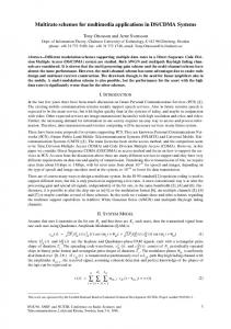
Fig. 1. Spanning subgraph k coloring (a) and induced subgraph k coloring (b) with k = 3, and minimum coloring (c) that requires k = 4. Numbers in the nodes are colors, with 0 meaning uncolored. The broken line marks an improperly colored edge.
creasing the network size (the number of connections) to . neurons would suffice, but no one has come In principle up with such an encoding. Our -state neuron approach originates from the idea that is more natural for a neuron to assume one of the states that represent the colors. This eliminates the possibility of conflicts among neurons in the same cluster and allows a more compact network representation with size of . the order of The main benefit of our approach in this paper is that it provides a generic methodology for deriving heuristic algorithms for difficult problems from energy functions in a largely problem-independent manner. Using this methodology on particular energy functions yields particular heuristic algorithms, some novel. Additionally, like most of the neural-networkbased algorithms, ours are intrinsically easy to parallelize [32], especially on SIMD parallel computers [10], [23]. Finally, using these methods for solving difficult optimization problems it is easy to tradeoff solution quality versus execution time. In this paper, in addition to the minimum coloring (MC) problem [Fig. 1(c)], we also solve two other important variants: • The spanning subgraph -coloring (SSC) problem is to minimize the number of improperly colored edges while coloring all the vertices in the graph using at most colors [Fig. 1(a)]. • The induced subgraph -coloring (ISC) problem is to find the largest set of vertices that can be properly colored using colors, possibly leaving some vertices in the graph uncolored [Fig. 1(b)]. We will also use SSC and ISC to approximately solve minimum coloring by using a binary search to select the number of colors . This paper is organized as follows: after a brief survey of the previous work in Section II, we describe the quasi-Hopfield optimizing neural network approach in Section III and propose and analyze three simple energy functions for the three graph coloring problems in Section IV. Then we detail the algorithm and the implementation in Section V and, finally, we report experimental results on benchmark graphs and a comparison with other methods in Section VI.
IEEE TRANSACTIONS ON NEURAL NETWORKS, VOL. 13, NO. 1, JANUARY 2002
II. RELATED WORK After the work by Hopfield and Tank [19], [20] several researchers have addressed the issue of mapping optimization problems onto neural networks. In particular, a number of solutions have been proposed to solve the graph coloring problem. The earliest efforts were focused on solving the four-colorability problem of planar graphs. Dahl [7] builds a neural network where neurons corresponding to the colors are asregions in the map. An energy funcsigned to each of the tion consisting of three terms is then minimized using a gradient descent dynamic. In order to avoid local minima and improper coloring, the value of three parameters requires adjustment according to the map size. Philipsen and Stok [36] transform the graph coloring problem into the maximum weight stable set problem, building an augmented graph with a clique of vertices (where is the maximum degree of the graph plus one) for each vertex of the original graph. To enforce feasibility of the solution, they use a previous approach proposed by Peterson and Soderberg [34] based on the mean field theory Potts neuron. Takefuji and Lee [40] use a Hopfield network with binary neurons to solve the four and -coloring problem of planar geographical maps. Their algorithm was later modified by Gassen and Carothers [15] to deal with the more general problem of generic graph -coloring, applied to register allocation optimization. Their modification includes a minimization term to reduce the number of colors used. Another extension to the -coloring problem of the Takefuji and Lee algorithm was later devised by Berger [1], who modified the energy function in order to guarantee convergence without resorting to the heuristic trimming of parameters necessary to the original algorithm. Later, Jagota [22] proposed a reduction of the coloring problem to the maximum independent set problem, followed by a mapping onto a Hopfield network. The network would then evolve using a dynamic algorithm called discrete descent, that had been used in earlier works to solve the maximum clique problem [21], [23], and that is also adapted to the modified approach presented in this paper. An interesting network-based algorithm that also encodes the color of a vertex in the state of a single cell is described in the work by Wu [41]. An array of coupled oscillators is considered as a graph by associating the oscillators to the vertices and couplings to edges. When the array is synchronized, the phase in each oscillator can be considered as the color of the corresponding vertex. There are several other approaches to the graph coloring problem that do not make use of neural networks [2]–[4], [6], [11], [12], [16], [17], [35], [24], [26]–[28], [31], [33], [38]. The last three of these, which we believe represent the state-of-the-art, will be briefly described in Section VI and compared with our results.
Given an undirected graph we build a corresponding neural nodes. An adjacency matrix has elenetwork composed of if otherwise. Each node has an ments output that corresponds to its state , and receives as input the states of all its neighboring nodes. A specific energy function is defined, based on the specific problem. The goal of the algorithm is to minimize the energy. We will update the network serially, specifically at time a single neuron will be selected and its state set to a new value such that (1) Thus, the energy will decrease in every time step. So long as the energy function is bounded from below, the network will always converge to a (local) minimum, that is, the network is globally stable. IV. ENERGY FUNCTIONS In this section we propose an energy function for each of the three graph coloring problems mentioned above. For each of them, we give the energy difference according to (1). We then analyze these energy functions to show that they exhibit some desirable properties. In particular we show that the solutions found are feasible and locally optimal, and that lower energy minima yield better solutions. For the spanning subgraph -coloring problem we propose the energy function
(2)
denotes a color assignment to all verwhere . The function is tices of from the set of colors a Kronecker delta function (in a slightly different notation) defined as if otherwise integers. Here we see that the energy function in (2) with simply represents the number of violations, that is, the number , for any given of improperly colored edges. Since a (local) minimum (locally) minimizes the number corresponds to a properly colored of violations and graph. For the induced subgraph -coloring problem we propose the energy function
III. THE NEURAL NETWORK Here we propose a multivalued neural network, where the different state of each neuron can assume one of or or . values, that is
(3)
DI BLAS et al.: ENERGY FUNCTION-BASED APPROACHES TO GRAPH COLORING
where it is important to note that now , where will denote that vertex is not colored. The function is the sign function, defined as if if if
83
For the MC energy function (4)
(7)
The (first) constraint term of (3) represents the number of imterm so that properly colored edges. We introduce the uncolored vertices do not generate improperly colored edges. The (second) objective term represents the number of colored vertices, regardless of their color value. Minimizing this energy function, therefore, means trying to minimize the number of improperly colored edges and at the same time trying to maximize conthe number of colored nodes. A balance parameter trols the tradeoff between these two terms. For the minimum coloring problem we propose the energy function
(4)
. Note that uncolored nodes are not alwhere lowed. Also note that has to be sufficiently large so that a proper coloring of the entire graph is feasible; for instance, we , where is the maximum degree can set balances the constraint term of miniin the graph. Here mizing the number of improperly colored edges with the objective term of minimizing the number of colors used. 1) Energy Difference: At each time step we compute the energy differences to implement the serial update so as to satisfy (1). We now compute the energy differences for the three energy functions. For the SSC energy function (2)
if and only if one of the following holds: 1) Here, , recoloring node with increases the number when or 2) when , of violations by less than recoloring node with reduces the number of violations by . Notice that in both cases one is trading off more than quality of the coloring versus the number of improperly colored edges. 2) Feasibility: We now show that the local minima of these three energy functions represent only feasible solutions of their associated problems. In the ISC and MC problems we will need to impose specific conditions on the parameter for this purpose. In the case of SSC, any coloring, even an improper one, is feasible, as long as all vertices are colored. In our encoding this . is always the case because of our choice In the case of ISC, a feasible coloring is a coloring that has no improperly colored edges. Intuitively, we see that when is large, a local minimum does not necessarily correspond to a feasible solution, i.e., some violations may be present, and that when is small all local minima correspond to feasible such that for solutions. Here we determine a critical value every local minimum is feasible. This value is critical in the sense that we will show a local minimum state in a graph that is not feasible. with all minima of the ISC energy Lemma 1: When function (3) are feasible solutions. Proof: A state is a minimum of the energy function (3) when no possible serial update can decrease the energy. Therefore, from (6)
(5) (8) if and only if assigning color to node Here, reduces the number of improperly colored edges among those touching node . For the ISC energy function (3)
(we drop the time must hold dependency for simplicity). Let us rewrite (8) as follows: (9) where
(6) if and only if one of the folHere, for lowing holds: 1) node is uncolored and coloring it increases the number of violations less than or 2) node is colored and recoloring it reduces the number of violations. if and only if node is colored and For uncoloring it reduces the number of violations by more than .
Here, represents the number of edges among those touching node that would be colored improperly if node were colored the number of edges among those
84
IEEE TRANSACTIONS ON NEURAL NETWORKS, VOL. 13, NO. 1, JANUARY 2002
such that
, and (11)
implies (a)
(b)
Fig. 2. An infeasible coloring that is a local minimum for the ISC energy function when (a) k = 1 and = = 1 and (b) an infeasible coloring that is a local minimum for the MC energy function when = = 1=2.
touching node that are colored improperly in the present represents the change in the total number of state, and colored nodes that would occur if node were (re)colored . hence, from (9) For (10) , (10) implies . Now, if then since it is an integer, and there are no violations in . Thus, we have shown that when every state which is a local minimum is feasible. To prove that this value is critical, we need simply offer an example: a graph is two nodes connected [Fig. 2(a)]. If , then by an edge, and a state in which both nodes are colored 1 is a local minimum , on the other hand, the network will but is infeasible. If converge to a state where one of the nodes is uncolored and the coloring is feasible. A feasible solution of the MC problem requires all nodes to be colored properly. Once again, it is easy to see that when is large, a local minimum will not necessarily be feasible, and when is sufficiently small all local minima are feasible. such As in the ISC case, we can compute a critical value we are guaranteed that every local minimum is that if a feasible solution. all minima of the Lemma 2: When MC energy function (4) are feasible solutions. Proof: This proof is similar to that of Lemma 1. In a local minimum the following holds from (7): Since
(11) where
and (12) represents the number of edges among those Here too, touching node that would be colored improperly if node were colored the number of edges among those touching node that are colored improperly in the present state, is the change in the objective function. and In a local minimum, the graph will be colored with . Therefore, colors from 1 to , with
(13) , if then Since . As in the ISC case, the value is critical. As an example, consider a three-node graph completely connected and . A state in which [Fig. 2(b)], where two nodes are colored 1 and the third node is colored 2 has one , this state is a local minimum. violation. However, if , the energy function will conOn the other hand, if verge to a feasible state where either one of the nodes that are colored 1 is recolored 3. 3) Local Optimality: Feasible solutions can be arbitrarily poor. For instance, in SSC a graph where all nodes are assigned the same color is feasible under the above definition, or, for ISC, a completely uncolored graph is feasible. Clearly these solutions are poor. However, it will turn out that the local minima of our energy functions will not only be feasible, but also locally optimal according to the definitions below. First we will define a to be a neighbor of state if state and , that is if and differ in exactly one component. Definition 1: A minimal-violations -coloring is a (not necof all nodes in essarily proper) coloring such that no coloring that is a neighbor of has fewer violations. in Definition 2: A maximal -coloring is a coloring of is properly colored and this coloring which a subset such that is not extendible, that is colored is a proper coloring. Definition 3: A minimal coloring is a proper coloring of all the nodes in such that for every proper coloring that is a neighbor of , where is the number of colors used in state . From the SSC energy function (2) it follows immediately that every local minimum yields a minimal-violations coloring. , every local minSimilarly, in the case of ISC, when imum of the energy function (3) yields a maximal -coloring. , It turns out that also in the case of MC, when local minima of the energy function (4) are minimal colorings. However, this is not immediately intuitive to see from the energy function definition as in the SSC and ISC cases. Therefore we have the following. Lemma 3: Every local minimum of the MC energy function is a minimal coloring. (4) with . Let Proof: Let be a local minimum with denote the number of nodes colored in state . We will prove by contradiction that is a minimal coloring. Let be a neighbor of that is also a proper coloring, and let . Let be the component in us suppose that which differs from . Let and . Since . Since is a local minimum, all , where colors of value less than are represented in is the set of nodes connected by an edge to node . Now, conused in . Any node colored is also sider any color
DI BLAS et al.: ENERGY FUNCTION-BASED APPROACHES TO GRAPH COLORING
in (if not, then could be recolored , which would imply that is not a local minimum). Hence, every color used in except is represented in . Thus would imply has violations, which contradicts assumption. 4) Representability: We have seen that all local minima for the three problems yield locally optimal solutions. It turns out that for the SSC and ISC problems the converse is also true— every locally optimal coloring is represented as a local minimum of the energy function. We call this property representability. Specifically, we note the following. • Every minimal-violations -coloring is represented in some local minimum of the SSC energy function. • Every maximal -coloring is represented in some local minimum of the ISC energy function with On the other hand, it is not true that every minimal coloring is represented in a local minimum of the MC energy function with . For instance a graph with two nodes connected by an edge where the nodes are colored one and three is a minimal coloring but not a local minimum. 5) Order Preservation: In mapping an optimization problem to an energy function, another desirable property is that lower minima of the energy function yield strictly better solutions of the problem, i.e., where and are two local minima states and is the quality of solution . A feasible mapping with this property is said to be order-preserving. One reason why the order-preserving property is a useful one is that if a mapping is feasible, representable, and order-preserving, then global optima of the energy function correspond to globally optimal solutions of the mapped problem. An even more practical value of the order-preserving property is based on the fact that one is rarely able to find an optimal solution, especially when the problem is NP-hard. Thus, since one will usually go only for local energy minima, the order-preserving property implies that deeper minima yield better solutions, while a mapping that preserves global optima might not be a useful one unless it is also order-preserving. We now discuss the three mappings from this perspective. First we need to define a measure of solution quality. For the SSC problem we will define this as the number of properly colored edges, for the ISC problem as the number of colored nodes, and for the MC problem as the negative of the number of distinct colors used. It can be easily seen that both the SSC and the ISC mappings are order-preserving. Unfortunately, the MC mapping (4) is not order-preserving since lower energies do not necessarily correspond to colorings that use fewer colors (Fig. 3). An idealized variant of this mapping, however, is almost order-preserving in the following sense: for any two states . Specifically, we generalize the MC energy function (4) to (14)
denotes the weight of color and is the number where of components colored in . With , (14) reduces to (4).
85
Fig. 3. Example of nonorder-preservation (not even almost orderpreservation) for MC: both states are minima with E (S~ ) = 9 < E (S~ ) = 10 , but Q(S~ ) < Q(S~ ) since S~ has three colors and S~ has two.
Lemma 4: With a feasible mapping of MC with regard to (14) is almost order preserving. Proof by Contradiction: In a feasible mapping, let and be two local minima, and suppose (if no such minima exist, the mapping is trivially order-preserving). Let and represent the highest color values used in and , . Then respectively, and suppose
since Furthermore,
Finally, since
and since there are no gaps in the coloring .
and both minima are feasible
We have a contradiction. Earlier, Korst and Aarts [29] encoded the MC problem to a Boltzmann machine with binary neurons (we use multivalued neurons). They obtained an analog of Lemma 4 in which they . It turns out that defined recursively in terms of Lemma 4 is asymptotically equivalent to their condition, while the proof above is simpler. Neither mapping is practical, though, grow exponentially with . Like Korst and since the weights Aarts, we will take a pragmatic approach. In particular, we will . We will see go back to our original encoding (4) with that the network using (4) finds good solutions, comparable in quality to the ones found by state-of-the-art methods. V. THE ENERGY MINIMIZATION ALGORITHM Here we describe a generic energy minimization algorithm applicable to the mapping of all three problems. The algorithm has two nested loops, an inner loop and an outer loop. The inner loop starts from a certain initial state and serially updates states until a minimum is reached. The outer loop repeatedly restarts the inner loop from different, randomly chosen, initial states and outputs the best solution found in any restart. The value of the outer loop is in compensating for the limited optimization ability of the inner loop by using multiple restarts. In the case of the ISC and MC problems, an intermediate loop will also perform an annealing of the parameter , interpreted as a temperature. Annealing will permit occasional uphill moves to escape local minima.
86
IEEE TRANSACTIONS ON NEURAL NETWORKS, VOL. 13, NO. 1, JANUARY 2002
Fig. 4. The inner loop.
1) The Inner Loop: At each time step, the color of one node is changed to reduce energy. When no change can further reduce energy, a local minimum is reached and the loop ends. At each time step, the node whose color is to be changed and the new color are picked as (15) is the matrix of for all pairs and where is any function of this matrix that returns some neuron-color satisfying when this is possible and pair when this is not. When , recoloring node with will necessarily reduce energy. The pseudo-code of the inner loop is shown in Fig. 4. to embody difWe can make different choices of ferent heuristics. Note that all will reduce energy. Let . Reasonable choices of include: with the minimum • greedy: returns the pair ; value of with equal • random: returns any random pair probability; returns a pair with • probabilistic-greedy: probability In all cases, will return if is empty. , rather than computing The subroutine from scratch as does , creates the by updating the old . This results in a significant new . We will distinguish two speedup over cases: 1) update , the row of corresponding to node that has just changed color, and 2) update for all nodes adjacent to node in . Rows in of nonneighbors of will not need updating. Let us first consider case 1). Our goal is to compute for all possible colors . Rather than recomputing all values from scratch, we can compute them as the sum of their previous value ) and the variation caused by the recoloring of node (at time at time , the delta energy variation, as in
to indicate the color of node at time , to avoid confusion. For the SSC energy function, from (5)
For the ISC energy function, from (6)
For the MC energy function, from (7)
Note that none of the depend on . Thus, while may be different for different colors , a the values single value is used to update them from their previous values. Using this idea, the complexity of computing the vector is reduced from using (1) to using (16). ’s of all Let us now consider case 2), the update of the node ’s neighbors. As in the previous case, we compute the variation in the delta energies for all possible colors in each . node For SSC, from (5)
for ISC, from (6)
(16) therefore reduces to computing Computing for all colors . From (16)
To compute this delta energy variation for SSC, ISC, and MC we consider that , since only node has been rather than recolored. In the following equations, we use
and for MC, from (7)
Therefore, the computational complexity of computing the vec’s of all neighbors of node is reduced from tors in the worst case using (1) to using (16).
DI BLAS et al.: ENERGY FUNCTION-BASED APPROACHES TO GRAPH COLORING
87
Fig. 5.
The annealing loop performed in the ISC and MC programs. In the SSC program, the annealing loop reduces to calling the inner loop function.
Fig. 6.
This function is used to set the value of .
Fig. 7.
The multiple-restarts outer loop.
2) The Annealing Loop: In the ISC and MC cases, the multiplier in (3) and (4) may be used to play the role of a temperature. Large values of permit uphill moves in the landscape of the energy function of small . In the ISC case, when is large more vertices may be colored at the expense of some edges becoming improperly colored. In the MC case, when is large a vertex colored with a high-valued color may be recolored with a lower-valued color (possibly reducing the total number of colors used) even at the expense of some edges becoming improperly colored. These observations suggest that we include in our algorithm an annealing loop. After experimentation we decided upon the algorithm in Fig. 5. and , are passed from the outside, with Two values of in the feasibility region and in the infeasibility region. The annealing loop first finds a proper coloring (using ) and then follows a two-step schedule in which and are used alternatively while the solution quality keeps improving. When the quality of the solution found is not better than in the previous iteration, the loop ends and returns the best solution found. and play a fundamental role. The In this procedure, must be less than to obtain a proper coloring, but value of
experimentally the energy descent evolution is almost insensitive to its specific value. Therefore, the value of can be computed directly. For example, in the ISC case we can set and in the MC case we can set . On the other hand, the annealing procedure is strongly sensi. When is small, the uphill moves tive to the value of permitted are limited, and the probability of reaching a different, lower proper minimum in the subsequent energy descent is large, too many uphill moves are permitted, is small. When and too much information related to the previous proper coloring is lost. Our heuristic is based on the idea of improving the current solution by permitting a large number of uphill moves while still preserving much of the current feasible state. we introduce the function To set the value of , whose pseudocode is shown in Fig. 6. This function is invoked in the outer loop (Fig. 7) before the first call to the annealing loop. In the ISC case, for a certain value of , the first proper coloring will color a certain fraction of the nodes. To implement the heuristic, we simply keep increasing the value of (in increments of value ) until all nodes are colored. The first . The value of for which this happens will be used as
88
IEEE TRANSACTIONS ON NEURAL NETWORKS, VOL. 13, NO. 1, JANUARY 2002
TABLE I SSC AND ISC PROGRAMS ON SOME OF THE DIMACS COLORING BENCHMARK GRAPHS. IN SSC, v IS THE NUMBER OF VIOLATIONS AND IN ISC n IS THE NUMBER OF COLORED NODES. THE VALUE OF k IS SET EQUAL TO OR TO ITS BEST KNOWN APPROXIMATION (IN PARENTHESES). TIMES ARE IN SECONDS (t[s])
function in the ISC case will return a TRUE in the value only if all nodes are colored. The increment ISC case will be set to one. This is justified by the fact that the number of violations that are permitted for coloring a (6). previously uncolored vertex is equal to the value of Therefore increments of less than a unit do not increase the possibility of uphill moves. In the MC case, after the first proper coloring, we increase the value of until the number of distinct colors used decreases below a certain fraction of the colors used in the first coloring , for instance). In the MC case, therefore, the function ( requires both the current state and the ini. The increment in the MC case is tial feasible state . From (7) and the proof of Lemma 2, we set to the value the number see that when increasing of an amount of violations allowed for recoloring vertices with lower color values will increase by at least one. 3) The Outer Loop: Fig. 7 shows the pseudocode for the outer loop. At each restart, based on the value of , the nodes’ states are randomly initialized and then the annealing loop function is called. If the solution found is better than the previous
best, it then becomes the new current best solution. The algorithm eventually outputs the best solution found. VI. EXPERIMENTAL RESULTS Our programs (SSC, ISC, and MC) were written in C, comcompiler (-O3 optimization) and run piled with the GNU on a 466 MHz Alpha. The programs were tested on the official benchmarks from the 1993 DIMACS graph coloring challenge [18], [25]. These graphs include several random graphs (DSJCx.y), geometric random graphs (DSJRx.y and Rx.y[c]), “quasirandom” graphs (flatx y 0), graphs from real-life applications (fpsol2.i.x, inithx.i.x, mulsol.i.1, and zeroin.i.1 map register allocation problems, school1 and school1 nsh are class scheduling graphs), graphs mapping combinatorial problems (queenx y), and artificial graphs (mycielx, lex y). For the selection function , with multiple random restarts a greedy, steepest-descent selection yields the best results in the case of SSC. In the cases of ISC and MC, we use different selection functions in different steps of the annealing. Even though single results may exhibit variations, the best combination appears to be the use of a greedy selection when the goal is to reach
DI BLAS et al.: ENERGY FUNCTION-BASED APPROACHES TO GRAPH COLORING
89
TABLE II RESULTS FROM SSC- AND ISC-BASED ALGORITHMS (SSC-B AND ISC-B, RESPECTIVELY) FOR MINIMUM COLORING, AND RESULTS FROM MC. TIMES ARE IN SECONDS (t[s]) OR, WHEN LONGER THAN ONE HOUR, IN HOUR: MINUTE FORMAT
a feasible minimum , and a random selection when the . goal is to move uphill and escape the local minimum A randomized-greedy selection function works about as well in either step, but is slightly slower in execution. 1) Spanning and Induced Subgraph Coloring: Table I reports averaged results over multiple runs of the SSC and the ISC programs. In both programs, the number of colors allowed is indicated in the column. The value of was set to when known. We did this to make the problems hard yet fully solvable, to permit evaluation of results. When was not known, was set to the cardinality of the smallest known coloring we were able to find in the literature (values in parentheses). The for the SSC program, total number of restarts was set to which does not perform annealing. For the ISC program the total number of restarts was set to 20 for all graphs. The results exhibit a large variation in solution quality. This is expected because the test graphs are significantly different from each other and they were created with “difficult to color” characteristics for the DIMACS challenge. However, in most instances, SSC colors more than 98% of the edges properly and ISC colors more than 85% of the nodes properly.
2) Minimum Coloring: In Table II we compare our three algorithms on the minimum coloring problem on the same graphs as in Table I. A minimum coloring can be found using SSC and ISC algorithms by adapting them to perform a binary search starting at . The names SSC-B and ISC-B indicate the binary search versions of SSC and ISC, respectively. The maximum number of restarts allowed at each stage of the for SSC-B and 20 for ISC-B, while the MC search was program was run with 10 restarts. The MC algorithm consistently performs better than SSC-B and ISC-B, even if allowed a smaller number of restarts. 3) Comparison With Other Methods: Finally, Table III compares MC with other algorithms reported in the literature (all timings are from the respective papers). The recursive binary adaptation (RBA) algorithm proposed by Jagota [22] is the only other neural algorithm for which we have results on DIMACS benchmarks. All the other neural approaches to the minimum coloring mentioned in Section II either do not offer experimental results or their test graphs are not available. Timings for RBA are on a SUN Sparc 10. “Coud” is the sequential coloring algorithm as modified by Coudert [4], probably the most efficient approach to date to
90
IEEE TRANSACTIONS ON NEURAL NETWORKS, VOL. 13, NO. 1, JANUARY 2002
A COMPARISON
OF
TABLE III MC WITH OTHER NEURAL (RBA) AND NON-NEURAL APPROACHES TO GRAPH COLORING. TIMES ARE (t[s]) OR, WHEN LONGER THAN ONE HOUR, IN HOUR: MINUTE FORMAT
graph coloring. It must be noted, however, that this algorithm works exceptionally well only on 1-perfect graphs, i.e., in which is equal to the size of the maximum clique. On other graphs (like the Mycielski transformation based graphs) it is as slow as a sequential “branch and bound” coloring. “Coud,” however, is an exact algorithm, always yielding an optimal coloring. Timings for “Coud” are on a 60 MHz SUN SuperSparc. “lmXRLF” is the least constraining-most constrained eXtended RLF algorithm by Kirovski and Potkonjak [28] that is based on the recursive largest first (RLF) heuristic by Leighton [30] to improve the simple sequential coloring. In this case we report only the coloring found, since they do not provide detailed timings but only state that none of the runs took longer than 1.5 hours and that all real-life examples were solved in less than a second on a SUN Sparc 5. “SWO” is the “Squeaky Wheel” Optimization algorithm by Joslin and Clements [26], a general approach to optimization based on the iterative application of a greedy algorithm and a solution analyzer that changes the priority in which the elements are considered by the greedy algorithm in the next iteration. Times for “SWO” are from a 333 MHz Pentium Pro. Finally, “DSATUR” is the well-known greedy routine by Brélaz [2]. We used the code provided by Joseph Culberson compiler and run on the same [5], compiled with the GNU 466 MHz Alpha that we used to run our MC program on.
IN
SECONDS
The nonneural algorithms specifically developed to solve the graph coloring problem tend to perform better than the neural ones. However, we see that no algorithm wins consistently, and that our implementation can still perform better than the other ones in some cases. VII. CONCLUSION We described a generalized quasi-Hopfield network approach to optimization that provides an algorithmic framework in which the problem-specific issues are embedded only in the energy function that the network evolution tries to minimize. We applied this approach to the solution of a family of NP-hard graph coloring problems, specifically the minimum coloring problem, the spanning subgraph -coloring problem and the induced subgraph -coloring problem. The use of multivalued neurons allowed a network representation that is more natural and compact than in previous simto ilar approaches. This reduced the network size from connections asymptotically and eliminated the possibility of conflicts among neurons in the same cluster. Experimental results showed that the performance of such a method compares favorably with other neural and nonneural approaches to the graph coloring problem. While acknowledging that the nonneural algorithms performed better on average on
DI BLAS et al.: ENERGY FUNCTION-BASED APPROACHES TO GRAPH COLORING
this specific problem, our approach retains its characteristics of generality that might make it successfully applicable to other optimization problems. Finally, due to its simple, clean structure, this approach is also intrinsically easy to parallelize. REFERENCES [1] M. O. Berger, “k -coloring vertices using a neural network with convergence to valid solutions,” in Proc. IEEE Int. Conf. Neural Networks, vol. 7, 1994, pp. 4514–4517. [2] D. Brélaz, “New methods to color the vertices of a graph,” Commun. ACM, vol. 22, pp. 251–256, Apr. 1979. [3] M. Chams, A. Hertz, and D. de Werra, “Some experiments with simulated annealing for coloring graphs,” Europ. J. Operational Res., vol. 32, pp. 260–266, 1987. [4] O. Coudert, “Exact coloring of real-life graphs is easy,” in Proc. 34th Design Automat. Conf.. New York, 1997, pp. 121–126. [5] Joseph Culberson’s Coloring Page, J. Culberson. [Online]. Available: http://web.cs.ualberta.ca/~joe/Coloring [6] J. C. Culberson and F. Luo, “Exploring the k -colorable landscape with iterated greedy,” in DIMACS Series in Discrete Mathematics and Theoretical Computer Science. Providence, RI: Amer. Math. Soc., 1996, vol. 26, pp. 245–284. [7] E. D. Dahl, “Neural network algorithm for an NP-complete problem: Map and graph coloring,” in Proc. IEEE Int. Conf. Neural Networks, vol. 3, 1987, pp. 113–120. [8] G. De Micheli, Synthesis and Optimization of Digital Circuits. New York: McGraw Hill, 1994. [9] D. de Werra, “An introduction to timetabling,” Europ. J. Operational Res., vol. 19, pp. 151–162, 1985. [10] A. Di Blas, A. Jagota, and R. Hughey, “Parallel implementations of optimizing neural networks,” in Proc. ANNIE 2000 Conf., Nov. 2000, pp. 153–158. [11] P. J. Donnelly and D. J. A. Welsh, The Antivoter Problem: Random 2-Colorings of Graphs. New York: Academic, 1984, pp. 133–144. Graph Theory and Combinatorics. [12] C. Fleurent and J. A. Ferland, “Object-oriented implementation of heuristic search methods for graph coloring, maximum clique and satisfiability,” in DIMACS Series in Discrete Mathematics and Theoretical Computer Science. Providence, RI: Amer. Math. Soc., 1996, vol. 26, pp. 619–652. [13] D. Gajski, N. Dutt, A. Wu, and S. Lin, High-Level Synthesis: Introduction to Chip and System Design. Boston, MA: Kluwer, 1992. [14] M. R. Garey and D. S. Johnson, Computers and Intractability: A Guide to the Theory of NP-Completeness. New York, NY: Freeman, 1979. [15] D. W. Gassen and J. D. Carothers, “Graph color minimization using neural networks,” in Proc. IEEE Int. Joint Conf. on Neural Networks, 1993, pp. 1541–1544. [16] F. Glover, M. Parker, and J. Ryan, “Coloring by tabu branch and bound,” in DIMACS Series in Discrete Mathematics and Theoretical Computer Science. Providence, RI: Amer. Math. Soc., 1996, vol. 26, pp. 285–308. [17] A. Hertz and D. de Werra, “Using tabu search techniques for graph coloring,” Computing, vol. 39, pp. 345–351, 1987. [18] Center for Discrete Mathematics and Theoretical Computer Science. [Online]. Available: http://dimacs.rutgers.edu [19] J. Hopfield and D. Tank, “Neural computation of decisions in optimization problems,” Biol. Cybern., vol. 52, pp. 141–152, 1985. , “Computing with neural circuits: A model,” Science, vol. 233, pp. [20] 625–633, 1986. [21] A. Jagota, “Approximating maximum clique with a Hopfield network,” IEEE Trans. Neural Networks, vol. 6, pp. 724–735, May 1995. [22] , “An adaptive, multiple restarts neural network algorithm for graph coloring,” Europ. J. Operational Res., vol. 93, pp. 257–270, 1996. [23] A. Jagota, L. Sanchis, and R. Ganesan, “Approximately solving maximum clique using neural network and related heuristics,” in DIMACS Series in Discrete Mathematics and Theoretical Computer Science: American Mathematical Society, 1996, vol. 26, pp. 169–204. [24] D. S. Johnson, C. R. Aragon, L. A. Mcgeoch, and C. Schevon, “Optimization by simulated annealing: An experimental evaluation; Part II, graph coloring and number partitioning,” Operations Res., vol. 39, pp. 378–406, May–June 1991. [25] D. S. Johnson and M. A. Trick, Eds., Clique, Coloring, and Satisfiability—Second DIMACS Implementation Challenge. Providence, RI: Amer. Math. Soc., 1996. [26] D. E. Joslin and D. P. Clements, “Squeaky wheel’ optimization,” J. Artificial Intell. Res., vol. 10, pp. 353–373, 1999. [27] D. Karger, R. Motwani, and M. Sudan, “Approximate graph coloring by semidefinite programming,” Proc. 35th IEEE Symp. Foundations of Computer Sci., pp. 2–43, 1994.
91
[28] D. Kirowski and M. Potkonjak, “Efficient coloring of a large spectrum of graphs,” in Proc. 35th Design Automat. Conf.. New York, 1998, pp. 427–432. [29] J. H. M. Korst and E. H. L. Aarts, “Combinatorial optimization on a Boltzmann machine,” J. Parallel Distributed Comput., vol. 6, pp. 331–357, 1989. [30] F. T. Leighton, “A graph coloring algorithm for large scheduling problems,” J. Res. Nat. Bureau Standards, vol. 84, no. 6, pp. 489–503, 1979. [31] G. Lewandowski and A. Condon, “Experiments with parallel graph coloring heuristics and applications of graph coloring,” in DIMACS Series in Discrete Mathematics and Theoretical Computer Science. Providence, RI: Amer. Math. Soc., 1996, vol. 26, pp. 309–334. [32] M. Misra, “Parallel environments for implementing neural networks,” Neural Comput. Surveys, vol. 1, pp. 46–80, 1997. [33] C. Morgenstern, “Distributed coloration neighborhood search,” in DIMACS Series in Discrete Mathematics and Theoretical Computer Science. Providence, RI: Amer. Math. Soc., 1996, vol. 26, pp. 335–358. [34] C. Peterson and B. Soderberg, “A new method for mapping optimization problems onto neural networks,” Int. J. Neural Syst., vol. 1, no. 1, pp. 3–22, 1989. [35] A. D. Petford and D. J. A. Welsh, “A randomised 3-coloring algorithm,” Discrete Math., vol. 74, pp. 253–261, 1989. [36] W. J. M. Philipsen and L. Stok, “Graph coloring using neural networks,” in IEEE Int. Symp. Circuits Syst., vol. 3, 1991, pp. 1597–1600. [37] S. Ramanathan and E. L. Lloyd, “Scheduling broadcasts in multihop radio networks,” IEEE/ACM Trans. Networking, vol. 1, pp. 166–172, 1993. [38] E. C. Sewell, “An improved algorithm for exact graph coloring,” in DIMACS Series Discrete Math. Theoretical Comput. Sci.: Amer. Math. Soc., 1996, vol. 26, pp. 359–373. [39] K. Smith and M. Palaniswami, “Static and dynamic channel assignment using neural networks,” IEEE J. Select. Areas Commun., vol. 15, pp. 238–249, Feb. 1997. [40] Y. Takefuji and K. C. Lee, “Artificial neural networks for four-coloring map problems and k -colorability problems,” IEEE Trans. Circuits Syst. I, vol. 38, pp. 326–333, Mar. 1991. [41] C. W. Wu, “Graph coloring via sinchronization of coupled oscillators,” IEEE Trans. Circuits Syst. I, vol. 45, pp. 974–978, Sept. 1998.
Andrea Di Blas (M’99) received the M.S. and Ph.D. degrees in electronic engineering from Politecnico di Torino, Italy, in 1994 and 2000. He has been a Researcher at University of California, Santa Cruz, since 1999, where he is currently also a Lecturer in the Department of Computer Engineering. His research interests include methodologies for parallel processing, neural networks, optimization problems, and bioinformatics.
Arun Jagota received the Ph.D. degree in computer science from The State University of New York, Buffalo. He has been a Visiting, Adjunct, or affiliated faculty member at the University of Memphis, the University of North Texas, the University of California, Santa Cruz, Santa Clara University, and San Jose State University. He has taught more than 35 different courses in computer science, and some in mathematics. He has authored more than 20 research papers in journals, and about the same number in conference records. He conducts research in neural networks, in machine learning, and in bioinformatics. Dr. Jagota is the Founding Editor of the journal Neural Computing Surveys. Richard Hughey (S’83–M’85) received the B.A. degree in mathematics and the B.S. degree in engineering from Swarthmore College, Swarthmore, PA, and the Sc.M. and Ph.D. in computer science from Brown University, Providence, RI. He is Associate Professor and Chair of the Department of Computer Engineering at the University of California, Santa Cruz. His research interests include parallel processing and bioinformatics. Dr. Hughey is a member of the American Society for Engineering Education (ASEE), the International Society for Computational Biology (ISCB), and the IEEE Computer Society.