Engineering Support Vector Machine Kernels That Recognize ...

E XTENDED A BSTRACT

Engineering Support Vector Machine Kernels That Recognize Translation Initiation Sites

A. Zien , G. R¨atsch
, S. Mika
, B. Sch¨olkopf
, C. Lemmen , A. Smola
, T. Lengauer , K.-R. M¨uller




GMD.SCAI, Schloss Birlinghoven, 53754 Sankt Augustin, Germany  zien, lemmen, lengauer  @gmd.de
GMD.FIRST, Rudower Chaussee 5, 12489 Berlin, Germany raetsch, mika, bs, smola, klaus  @first.gmd.de

Abstract In order to extract protein sequences from nucleotide sequences, it is an important step to recognize points from which regions encoding proteins start, the so-called translation initiation sites (TIS). This can be modeled as a classification problem. We demonstrate the power of support vector machines (SVMs) for this task, and show how to successfully incorporate biological prior knowledge by engineering an appropriate kernel function. 1 Introduction Living systems are determined by the proteins they produce according to their genetic information. But only parts of the nucleotide sequences carrying this information encode proteins (CDS, for coding sequence), while other parts (UTR, for untranslated regions) do not. Given a piece of DNA or mRNA sequence, it is most interesting to know whether it contains CDS, and, if so, which protein it encodes. In principle, both CDS and the encoded protein can be characterized using alignment methods. Programs capable of aligning nucleotide sequences to protein databases include FASTX/FASTY, SearchWise and BLASTX. However, this approach is hampered by two severe problems: First, there are several sources of noise making the task more difficult and errorprone than pure protein alignment: (i) The correct strand and reading frame have to be found. (ii) Additional false hits may result from UTR sequences. (iii) Sequencing errors may disrupt the correct reading frame. Second, alignment based approaches rely on homologous proteins being known. This renders them unapt to find

novel genes. Thus, a method to identify CDS in nucleotide sequences is desirable, both in order to ease the task for alignment-based approaches as well as to find new genes. Since living cells are able to distinguish between CDS and other nucleotide sequence parts without utilizing any homology information, this should in principle also be possible for computer programs. In fact, there are algorithms that identify CDS merely relying on properties intrinsic to nucleotide sequences. The most successful programs include GENSCAN [5] for genomic DNA and ESTScan [6] for ESTs. ESTs are single-read partial sequences derived from mRNA that are particularly errorprone. ESTScan implements a fifth-order hidden Markov model that simultaneously recognizes CDS by typical oligo-nucleotide frequencies and corrects sequencing errors. It does not incorporate a model of translation initiation site (TIS) sequences, that mark the beginning of CDS. GENSCAN employs generalized hidden Markov models to capture the structure of an entire genome. Despite its overall sophistication, GENSCAN uses a relatively crude TIS model: a piece of sequence is assigned a probability for being a TIS, based on the positional relative frequencies of individual nucleotides observed around a true TIS. There exists a number of more elaborate models of TIS themselves. Salzberg extends the positional probabilities (as used by GENSCAN) to first order Markovian dependencies [13]. This is essentially a proper probabilistic modeling of

positional di-nucleotides, and leads to a significant increase in recognition performance. There also exist methods to explicitly capture correlations between non-adjacent positions near TIS or other signals [1], possibly aiding insight into the structural functioning of these signals. However, since few such correlations can be proved to be significant in TIS sequences, there is little gain for TIS recognition. All models discussed so far can be called generative, as they can be used to generate potential TIS sequences with approximately the true probability distribution. Applying such models, a sequence is considered a TIS if the probability it is assigned exceeds some threshold. The more closely the true distribution is approximated, the better this approach works. By using so-called discriminative methods, in general a superior distinction between true and pseudo TIS can be achieved. These methods aim at learning to discriminate certain objects from others, without explicitly considering probability distributions. For example, the program ATGpr [12] uses a linear discriminant function that combines several statistical measures derived from the sequence. Each of those features is designed to be distinctive for true versus pseudo TIS. Learning allows to find a (linear) weighted combination of features that achieves a good discrimination. A radically different approach to learning a discriminating function is taken by Pedersen and Nielsen [11]. They train an artificial neural network (NN) to predict TIS from a fixed-length sequence window around a potential start codon (ATG). The input of the NN consists of a binary encoding of the sequence; no higher-level features are supplied. The intriguing idea is that the NN learns by itself which features derived from the sequence are indicative of a true TIS. Of the described methods, only ATGpr makes use of the ribosome scanning model [9]. According to this model, the translation starts at the first occurrence of an appropriate signal sequence in the mRNA, and thus sequences further downstream that resemble typical TIS are inactive (pseudo sites). The scanning model can be combined with any TIS recognition method, and is confirmed by the resulting improvements of recognition [2]. Since the model is orthog-

onal to TIS signal sequence recognition itself, and is limited to complete mRNA sequences, we will not consider it in the following. In this paper, we show that we can top the performance of established methods for TIS recognition by applying support vector machines (SVMs) [4]. Like NNs, SVMs are a discriminative supervised machine learning technology, i.e. they need training with classified data in order to learn the classification. For the task of TIS recognition, we show that SVMs can be superior to NNs. To achieve this performance gain we use a particularly desirable property of SVMs: the ability to adapt them to the problem at hand by including prior knowledge into the so-called kernel function. Here, we demonstrate how to make use of rather vague biological knowledge. The paper is structured as follows: we first give a brief description of the SVM technique, then present experiments and finally discuss results and potential applications. 2 Methods 2.1 Support Vector Machines Formally, SVMs like any other classification method aim at estimating a classification function using classified training data from such that will correctly classify unseen examples (test data). In our case, will contain simple representations of sequence windows, while corresponds to true TIS and pseudo sites, respectively. In order to be successful, two conditions have to be respected. First, the training data must be an unbiased sample from the same source as the test data will be. This concerns the experimental setup. Second, the size of the class of functions that we choose our estimate from, the so-called capacity of the learning machine, has to be sensibly restricted. If the capacity is too small, complex discriminant functions can not be sufficiently well approximated by any selectable function – the learning machine is too dumb to learn well. On the other hand, too large a capacity bears the risk of loosing the ability to learn a function that generalizes well to unseen data. The reason lies in the existence of infinitely many functions that are consistent with the training examples, but disagree on unseen (test) examples. Most of those functions per-

   

     









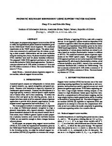
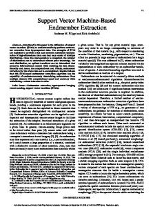
fectly memorize the particular examples used for training, but do not reflect general properties of the classification. Picking such a function is called overfitting. In neural network training, overfitting is avoided by early stopping, regularization or asymptotic model selection [3, 10]. In contrast, the capacity of SVMs is limited according to the statistical theory of learning from small samples [17]. For learning machines implementing linear decision functions this corresponds to finding a large margin separation of the two classes. The margin is the minimal distance of training points to the separation surface (cf. Figure 1). Finding the maximum margin separation can be cast as a convex quadratic programming (QP) problem [4]. The time complexity of solving such a QP scales approximately between quadratic and cubic in the number of training patterns (see [14]), making the SVM technique computationally comparably expensive. With respect to good generalization, it often is profitable to misclassify some outlying training data points in order to achieve a larger margin between the other training points. See Figure 1 for an example. This ’neglectful’ learning strategy also masters inseparable data [16], which is frequent in real-world applications. The tradeoff between margin size and number of misclassified training points is controlled by a parameter of the SVM, which therefore can be used to control its capacity. This extension still permits optimization via QP [4]. It is tempting to think that linear functions can be insufficient to solve complex classification tasks. A little thought reveals that this in fact depends on the representation of the data points. Canonical representations, as frequently used to define input space, tend to minimize dimensionality and avoid redundancy. Then, linearity may easily be too restrictive. However, one is free to define (possibly redundant) features that nonlinearly derive from any number of input space dimensions. Even for complex problems, well chosen features could ideally be related to the respective classification by rather simple means, e.g. by a linear function (cf. Figure 2). Any linear learning machine can be extended to functions non-linear in input space by



Figure 1: A binary classification toy problem: separate dots from crosses. The shaded region consists of training examples, the other regions of test data (spatial separation for illustration clarity only). The data can be separated with a margin indicated by the slim dotted lines, implicating the slim solid line as decision function. Misclassifying one training point (circled cross) leads to a considerable extension (arrows) of the margin (fat lines) and thereby to the correct classification of two test examples (circled dots).

explicitly transforming the data into a feature (see Figure space using a map 2). SVMs can do so implicitly, thanks to their mathematical niceness: all that SVMs need to know in order to both train and classify are dot products of pairs of data points in feature space. Thus, we only need to supply a so-called kernel function that computes these dot products. This kernel function implicitly defines the feature space (Mercer’s Theorem, e.g. [4]) via



  

!"$#% &

&')(+*,-./(0213*,45

Note that neither the SVM nor we need to know , because the mapping is never performed explicitly. Therefore, we can computationally afford very large (e.g. dimensional) feature spaces. SVMs can still avoid overfitting thanks to the margin maximization mechanism. Simultaneously, they can learn which of the features implied by are distinctive for the two classes. So, instead of having to design well-suited features by ourselves (which can often be difficult), we can use the SVM to select them from a sufficiently rich feature space. Of course, it well be helpful if the kernel supplies a type of features related to the correct classification. In the next sections, we will show how to boost the process of learning by choosing appropriate kernel functions.



&

7698!:

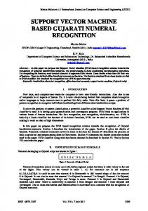
(a)

(b)

(c)

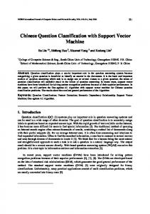
Figure 2: Three different views on the same dot versus cross separation problem. Linear separation of input points (a) does not work well: a reasonably sized margin requires misclassifying one point. A better separation is permitted by non-linear functions in input space (b), which corresponds to a linear function in a feature-space (c). Input space and feature space are related by the kernel function (see main text).

2.2 Data sets Little experience exists in the application of SVMs to biomolecular problems (to our knowledge, only work by Jaakkola and Haussler [8]). Therefore, we compare the performance of SVMs to that of the most popular alternative general purpose machine learning technology, neural networks (NNs). In order to do so, we use the vertebrate data set provided by Pedersen and Nielsen [11]. We take care to only replace the learning machinery while retaining the setting: the definition of training and test data sets as well as the definition of input space. The sequence set is built from high quality nuclear genomic sequences of a selected set of vertebrates taken from GenBank. All introns are removed, in analogy to the splicing of mRNA sequences. The set is thoroughly reduced for redundancy, to avoid over-optimistic performance estimates resulting from biased data. This protocol leaves 3312 sequences (see [11]). From these sequences, the data set for TIS recognition is built as follows. For each potential start codon (the nucleotide sequence ATG) on the forward strand, one data point is generated. This leads to 13503 data points, of which 3312 (24.5%) correspond to true TIS and the other 10191 (75.5%) correspond to pseudo sites. Each data point is represented by a sequence window of 200 nucleotides centered around the respective ATG triplet. Pedersen and Nielsen divide the data into six parts of nearly equal size points) and fraction of true TIS. Each ( part is in turn reserved for testing the classification learned from the other five parts.

;=