Equilibrium Approximation in Simulation–Based Extensive–Form Games Nicola Gatti
Marcello Restelli
Politecnico di Milano Piazza Leonardo da Vinci 32 Milano, Italy
Politecnico di Milano Piazza Leonardo da Vinci 32 Milano, Italy
[email protected]
[email protected]
ABSTRACT The class of simulation–based games, in which the payoffs are generated as an output of a simulation process, recently received a lot of attention in literature. In this paper, we extend such class to games in extensive form with continuous actions and perfect information. We design two convergent algorithms to find an approximate subgame perfect equilibrium (SPE) and an approximate Nash equilibrium (NE) respectively. Our algorithms can exploit different optimization techniques. In particular, we use: simulated annealing, cross entropy method, and Lipschitz optimization. We produce an extensive experimental evaluation of the performance of our algorithms in terms of approximation degree of the optimal solution and number of evaluated samples. Finding approximate NE and SPE requires exponential time in the game tree depth: an SPE can be computed in game trees with a small depth, while the computation of an NE is easier.
Categories and Subject Descriptors I.2.11 [Computating Methodologies]: Distributed Artificial Intelligence.
General Terms Algorithms, Economics.
Keywords Game Theory (cooperative and non-cooperative).
1.
INTRODUCTION
Non–cooperative game theory provides formal tools to model situations wherein rational agents interact and describes the pertinent solution concepts [5]. The central solution concepts are the Nash equilibrium for games in which agents play simultaneously (said in strategic form) and the subgame perfect equilibrium when agents play sequentially (said in extensive form). Game theory proves that any finite game admits at least an equilibrium (Nash and subgame perfect), however it leaves open the problem to compute it. Equilibrium computation is currently one of the most challenging problem in computer science [17]. Cite as: Equilibrium Approximation in Simulation–Based Extensive– Form Games, Author(s), Proc. of 10th Int. Conf. on Autonomous Agents and Multiagent Systems (AAMAS 2011), Tumer, Yolum, Sonenberg and Stone (eds.), May, 2–6, 2011, Taipei, Taiwan, pp. XXX-XXX. Copyright © 2011, International Foundation for Autonomous Agents and Multiagent Systems (www.ifaamas.org). All rights reserved.
The formal model of a game is based on the concept of mechanism. It defines the rules of the game, specifying the number of roles of the agents, the actions available to the agents, the sequential structure of the game, and the preferences of the agents over the outcomes (usually expressed as utility functions). Almost the entire game theory deals with games where the agents’ utility functions are known in analytical form. Recently, the class of simulation–based games have been proposed, in which the agents’ utility are not analytical known, but they are the result of a (usually continuous) simulation process. The main interest in studying these games lays in developing algorithms able to find agents’ (approximate) equilibrium strategies without having any information about the simulation process. The main work on equilibrium computation for simulation– based games is described in [21]. The authors provide algorithms based on best response iteration to find an approximate Nash equilibrium, where the best responses are approximated by using stochastic optimization techniques (precisely, simulated annealing). The authors discuss also the conditions that assure their algorithms to converge (in probability) to an equilibrium. However, this work is applicable only to games in strategic form. The study of simulation–based games in extensive form has not received enough attention. To the best of our knowledge, the unique pertinent result is provided in [20], where the authors employ the simulation–based framework for mechanism design. In this paper, we provide the first study of simulation– based (continuous) extensive–form games. After having defined the class of simulation–based extensive–form games (Section 2), we provide two algorithms to compute an approximate Nash equilibrium (NE) and an approximate subgame perfect (SPE) respectively, that work directly on the game tree (Section 3). These algorithms exploit black–box (stochastic) optimization techniques. We develop our algorithms with three different optimization techniques: simulated annealing (as in [21]), cross entropy method, and Lipschitz optimization. Then, we experimentally evaluate the performance of our algorithms (and optimization techniques) in terms of: ǫ value of the found ǫ-approximate equilibrium, number of evaluated samples, and time (Section 5). We experimentally show that an NE can be found in game trees deeper than in the SPE case.
2. SIMULATION-BASED AND EXTENSIVEFORM GAMES The class of simulation–based games was introduced in [21] and captures situations where the agents’ utility functions
u = E[O] is the underlying game of the simulation–based game where the oracle is O. Given u(t), we denote by ui (t) the component of u reporting the utility of agent i.
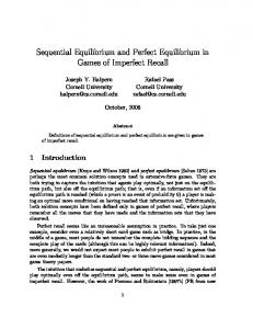
agent 1 (x1) 1
1
3
>.5 agent 2 (x2)
2
0
x2 .5
1
x2 .5
1
3
2
0
2.2 Strategies
0
0 0
.5 x1
1
0
.5 x1
1
u1(x1,x2),u2(x1,x2) u1(x1,x2)
u2(x1,x2)
game tree
Figure 1: A two–level continuous game with two agents: game tree (left), and agents’ utility functions (middle and right). are not analytically known, but they are given as the result of a simulation process. Formally, there is an oracle O that, given an outcome of the game, produces a (possibly noisy) sample from the agents’ joint utility functions. Since most of simulation processes are based on real–valued variables, a very interesting class of simulation–based games is that of games where the agents’ actions are continuous. In these games, the actions available to the agents are the assignment of values to one or more real–valued variables. In what follows, we define the concept of simulation–based extensive– form games and we review the appropriate solution concepts. As customary in game theory, we distinguish the mechanism, that specifies the game rules, from the strategies, that specify the agents’ behavior during the game.
2.1 Mechanism A finite perfect–information extensive–form game is a tuple (N, A, V, T, ι, ρ, χ, u), where: N is the set of n agents, A is a set of actions, V is the set of decision nodes of the game tree, T is the set of terminal nodes of the game tree, ι ∶ V → N is the agent function that specifies the agent that acts at a given decision node, ρ ∶ V → ℘(A) returns the actions available to agent ι(v) at decision node v, χ ∶ V ×A → V ∪T assigns the next (decision or terminal) node to each pair composed of a decision node v and an action a available at v, and u = (u1 , . . . , un ) is the set of agents’ utility functions where ui ∶ T → R. An extensive–form game is with imperfect–information when some action of some agent is not perfectly observable by the agent’s opponents. In this paper, we limit our study to perfect–information games. Furthermore, we focus on games with perfect recall, where every agent recalls all the previously undertaken actions. In our work, we consider continuous perfect–information extensive–form games. In these games, sets A, V , and T are compact. Given a decision node v, agent ι(v) has a continuous set of actions ⊆ A. Each action can lead to a different decision or terminal node. (The model can be easily extended to the case in which A, V , and T are mixed sets composed of continuous and discrete elements.) Example 2.1. Consider Figure 1, there are two agents (i.e., agent 1 and agent 2) that play according to a two–level game tree where the first agent to play is agent 1. Agent 1 can assign a real value to x1 from the range [0, 1]. After the assignment by agent 1, agent 2 can assign a real value to x2 from the range [0, 1]. Agents’ utility functions are defined on x1 and x2 as shown in figure. In a simulation–based extensive–form game, players’ utility functions u are not known. Formally, the component u in the tuple (N, A, V, T, ι, ρ, χ, u) is substituted by oracle O whose argument is t ∈ T . We say that (N, A, V, T, ι, ρ, χ, u) where
In an extensive–form game, a pure strategy σi is a plan of actions specifying one action for each decision node of agent i. A mixed strategy σi is a randomization over pure strategies (plans). When the game is continuous, the definition of a single plan is extremely complex and cannot be conveniently used. An alternative and more compact representation is given by behavioral strategies. These define the behavior of an agent at each node independently of the choices taken at other nodes. Essentially, a behavioral strategy σi assigns each decision node v ∈ V a probability distribution over the actions available at v. With perfect recall, the two representations (plans and behavioral) are equivalent. A strategy profile collects the strategies of all the agents and is defied as σ = (σ1 , . . . , σn ). With continuous games, behavioral strategies are usually expressed as functions that map actions played at previous nodes to an action (or a probability distribution) available at the current node. Example 2.2. Consider the game in Fig. 1, possible strategies for agent 1 and agent 2 are: σ1 = {x1 = .3 σ2 = {
x2 = .6 x2 = .9
if x1 ≤ .2 if x1 > .2
Solving a game means to find a strategy profile in which agents’ strategies are somehow in equilibrium. Under the assumption that information is complete and common we can define the concept of Nash equilibrium (NE) as a strategy profile σ such that for all i ∈ N : σi is a best response to σ−i where σ−i is given by σ once σi has been removed (easily, a strategy σi is a best response when no other strategy provides a larger utility). It is well known that in extensive– form games some Nash equilibria may be not reasonable with respect to the sequential structure of the game [5]. When information is perfect, the appropriate refinement of Nash for extensive–form games is the subgame perfect equilibrium (SPE) [5]. With perfect information, a subgame is a subtree of the game tree. Obviously, in continuous games, there are infinite subgames. A subgame perfect equilibrium is a strategy profile that is a Nash equilibrium in every subgame. Every finite extensive–form with perfect information has at least one subgame perfect equilibrium in pure strategies [5]. The same result holds when the game is continuous with bounded utility functions [8]. Since the subgame perfect equilibrium is a refinement of the Nash equilibrium, every continuous perfect–information extensive–form game always admits at least one Nash equilibrium (instead, continuous one–shot games may not admit any Nash equilibrium). Example 2.3. Consider the game depicted in Fig. 1. There is ‘essentially’ a unique SPE (rigorously speaking, there are infinite SPEs, but they are all equivalent in terms of utilities), represented in Fig. 2 where: σ1 = {x1 > .5 σ2 = {
x2 ≤ .5 x2 > .5
if x1 ≤ .5 if x1 > .5
This game does not admit additional NEs in pure strategies.
Algorithm 1 spe approximation(v) 1: if v is terminal then 2: return O(v) 3: else 4: {σk (v)} ← sample initialization(ρ(v)) 5: while true do 6: for each σk (v), assign uk = spe approximation(χ(v, σk (v)))
agent 1 (x1)
.5
agent 2 (x2)
.
>.
1,
5
1
.5
player 1 (x1)
player 2 (x2)
.
5
2,
1, 2
3,
3
.5
player 2 (x2) 5
5
1
.
1,
5
1
5
1
.5 when agent 1 play x1 = w with w > 0.5, to force agent 1 to play x1 = w with w ≤ 0.5. Since our aim is to approximate equilibrium strategies in simulation–based games, we resort to the concepts of approximate equilibrium. Several concepts are available in the literature: ǫ–close, ǫ–Nash, and ǫ–perfect equilibria. An ǫ– close equilibrium is a strategy profile σ in which the distance (according to some metric) between every σi and σi∗ is smaller than ǫ, where σi∗ is the optimal strategy of i in an NE σ ∗ . This concept provides a measure of the approximation degree of the strategy. However, it is usually considered non–satisfactory and it is preferred the provision of the approximation degree of the expected utility. An ǫ–Nash equilibrium is a strategy profile σ where no agent can improve more than ǫ her utility by a unilateral deviation, while an ǫ–perfect equilibrium takes into account also the deviations of the opponents at all the subgames.
3.
ALGORITHMS
The approximation of an equilibrium in simulation–based extensive–form games cannot be tackled with the algorithms proposed for strategic–form games. To use these algorithms, we need to represent the agents’ strategies as plans of actions and this is impractical.1 This pushes for the development of ad–hoc algorithms that work directly on the game tree. 1
Notice that the game cannot be solved by using the algorithm described [21] assuming that agent 1 and agent 2 assign values to x1 and x2 respectively. This would neglect the game sequential structure.
SP E
(v) = arg max uι(v) (χ(v, σ)) , SP E
σ∈ρ(v)
(1)
where uSP E (v) is defined as SP E
u
(v) = {
O(v) SP E SP E u (χ (v, σ (v)))
if v is terminal otherwise.
Algorithm 1 reports the pseudo–code to compute an approximate SPE. The algorithm, that works recursively, receives, as input, the current node v. Initially, the algorithm is called with v as the root node. If the current node v is terminal, then the oracle is called and a sample of agents’ utilities are returned (Line 2). Otherwise, the optimal strategy at v is searched as follows. Initially, one or more action samples are generated (Line 4). Then, each sample σ k (v) is evaluated by recursively calling spe approximation on the node reachable by application of action σ k (v) to node v (Line 6). Given the evaluation of all the samples, if a termination condition holds (Line 7), the largest utility among those of all the samples is returned (Line 8). Otherwise, new samples are generated (Line 11). Functions sample initialization, samples generation, and termination condition are based on black–box non–linear optimization techniques (their description is provided in Section 4). Example 3.1. Consider the game in Fig. 1. Algorithm 1 works as follows. At first some samples of x1 are generated, e.g., {.2, .4, .8}. For each sample, the algorithm is recursively called and samples for x2 are produced, e.g., {.3, .5, .8} for x1 = .2. Then, an iterative optimization process based on resampling is carried on to optimize the value of x2 (i.e., ≤ .5 for x1 = .2) and, finally, to return the evaluation of utility associated with the sample of x1 = .2 (i.e., u1 = 1). Once utility associated with all the generated samples of x1 are evaluated, an iterative optimization process based on resampling is carried on to optimize the value of x1 (i.e., u1 = 2). Provided that the black–box non–linear optimization technique converges to the global optimum (see Section 4.4), it is easy to show that the proposed algorithm computes the solution of problem in Equation 1.
Algorithm 2 ne approximation (v) 1: if v is non–preterminal then 2: σ(v) ← a random value uniformly distributed in ρ(v) 3: u ← ne approximation(χ(v, σ(v))) 4: while true do 5: [ˆ u, σ ˆ (v)] ← ne validation(v, v) 6: if u ˆι(v) ≤ u(v) then 7: return u 8: else 9: σ(v) ← σ ˆ (v) 10: u ← ne approximation(χ(v, σ(v))) 11: end if 12: end while 13: else 14: {σk (v)} ← sample initialization(ρ(v)) 15: while true do 16: for each σk (v), assign uk = O (χ(v, σk (v))) 17: if termination condition({σk (v)}, {uk }) then 18: return arg max uι(v) 19: 20: 21: 22: 23:
u∈{uk }
else {σk (v)} ← samples generation(ρ(v), {σk (v)}, {uk }) end if end while end if
3.2 Computing an approximate NE Surprisingly, although the NE concept poses constraints less hard than the SPE concept, the algorithm computing an NE results to be more twisted than the one computing an SPE. An NE can be formulated as in Equation 1 as far as the nodes on the equilibrium path are considered, while off the equilibrium path other agents may be non-maximizers. Algorithm 2 depicts the pseudo–code computing an approximate NE. In the computation of an NE, two phases can be recognized. During the first phase (entirely executed by Algorithm 2), a strategy profile σ, limited to the equilibrium path, is searched. During the second phase (mainly executed by Algorithm 3), a possible strategy profile off the equilibrium path is searched such that σ is an NE. Essentially, the second phase validates that σ is an NE. The two phases iteratively alternate during the execution until an approximate NE has not been found. The details follow. (First phase) In Algorithm 2, for each non–preterminal node2 v a random strategy is assigned to σ(v) (Line 2) and the algorithm is recursively called on the next node reached by applying σ(v) to the current node (Line 3). If v is preterminal, the best strategy of agent ι(v) at v is searched by using black-box optimization techniques (Lines 14–22). Notice that this optimization works exactly as Lines 6-13 of Algorithm 1 except that here the evaluation of the sample is directly accomplished by calling the oracle without any recursive call of the algorithm. Once Line 18 is executed, a complete strategy assignment σ from the root of the tree to a terminal node (along a single path) is built. Example 3.2. Consider the game depicted in Fig. 3. Algorithm 2 randomly assigns a value to x1, e.g., x1 = 0.3, and subsequently the optimal value of x2 is found, i.e., x2 ≥ .5. (Second phase) The algorithm tries to validate that the found strategy profile σ is an NE (Line 5). This is accomplished by Algorithm 3. Given a node v, Algorithm 3 searches for a strategy in the subgames such that agent ι(v) cannot gain more by deviating from her strategy prescribed 2
A node v is preterminal if, once applied an action to v, a terminal node is reached.
Algorithm 3 ne validation (v, v0 ) 1: if v is terminal then 2: return O(v) 3: else 4: {σk (v)} ← sample initialization(ρ(v)) 5: while true do 6: for each σk (v), assign uk = ne validation(χ(v, σk (v)), v0 ) 7: if ι(v) = ι(v0 ) then 8: if termination condition({σk (v)}, {uk ι(v) }) then k 9: return [arg max uι(v) , best σ (v)] 10: 11: 12: 13: 14: 15: 16: 17: 18: 19: 20: 21:
u∈{uk }
else {σk (v)} ← (ρ(v), {σk (v)}, {uk ι(v) })
samples generation
end if else if termination condition({σk (v)}, {−uk ι(v return [arg min uι(v0 ) , best σ (v)] k
0)
}) then
u∈{uk }
else {σk (v)} ← ples generation(ρ(v), {σk (v)}, {−uk ι(v ) })
sam-
0
end if end if end while end if
by σ. Differently from what happens in the case of SPE, the strategy in the subgames of v does not need to be sequentially rational. Practically, this means that, while agent ι(v) will maximize her utility in such subgames, the behavior of her opponents is free, they do not necessarily maximize their utility. To assure that there is not any strategy such that ι(v) can gain more by deviating form her strategy prescribed by σ at v, we assume that all the opponents of ι(v) behave in the attempt to minimize the utility of ι(v). In this way, we find the maxmin value of agent ι(v) from the subgames. If the maxmin value is larger than the utility given by the strategy prescribed by σ, then σ is not an NE, otherwise there is at least a strategy of the subgames such that the strategy prescribed by σ is optimal. The validation process must be repeated at every node v. If a strategy is not validated at a given node v, Algorithm 2 assigns the maxmin strategy of the subgames to σ(v) (Line 8) and phase 1 is restarted. Algorithm 3 works similarly to Algorithm 1 except that the opponents of agent ι(v0 ), where v0 is the node whose strategy we are validating, minimize agent ι(v0 )’s utility (Line 15). We use the same black–box optimization techniques used in the previous algorithms, passing {−ukι(v0 ) } when we need to minimize (Lines 14 and 17). Example 3.3. Consider the game depicted in Fig. 3. Suppose that Algorithm 2 has assigned x1 = .3 and x2 = .1, and that ne validation is executed to validate the strategy of agent 1. A number of samples are generated for x1. For each sample of x1, the optimal value of x2 minimizing agent 1’s utility is found. It can be easily observed that the maxmin utility of agent 1 from all the subgames is 1 and therefore the initial strategy is validated. The efficiency of Algorithm 3 can be improved by using a pruning procedure similar to the alpha–beta pruning. More precisely, call v0 the node whose strategy is to validate. To assert that a given strategy σ is not an NE, we do not need to compute the maxmin value of v0 , but it is enough to find a strategy σ ˆι(v0 ) such that agent ι(v0 )’s utility is larger than
the one provided by the strategy to validate. Moreover, in all the subgames of v0 , we do not strictly need that opponents of agent ι(v0 ) find the minimum of agent ι(v0 )’s utility, but it is sufficient that they find an action such that agent ι(v0 )’s utility is not larger than the one provided by the strategy to validate. Therefore, the termination condition at Line 8 can be safely modified in the following way: as soon as a sample provides agent ι(v0 ) with a utility larger than the one provided by the strategy to be validated, the algorithm returns such utility and the corresponding sample. Similarly, at Line 14 it is possible to make the algorithm return as soon as a sample, that provides agent ι(v0 ) with a utility non– larger than the one provided by the strategy to be validated, is found. Example 3.4. Consider Example 3.3. Every time a sample of x2 is evaluated and it provides a utility of 1 to agent 1, no further samples are generated.
4.
OPTIMIZATION ALGORITHMS
As shown in the previous section, the computation of an SPE and an NE in extensive–form games requires to solve a number of recursive optimization problems. For each node v we need to maximize an unknown objective function which depends on the solutions of other optimization problems defined in the nodes of the sub–tree rooted at v. In a continuous extensive–form game, this means to solve a number of unconstrained continuous optimization problems. In the literature, researchers have proposed many optimization methods, which can be split into two main categories: deterministic methods (e.g., real algebraic geometry [2], Lipschitz optimization [18]) and non–deterministic (or stochastic) ones (e.g., evolutionary algorithms [7], simulated annealing [10], cross-entropy method [16], particle swarm optimization [9]). The optimization process which is common to all these algorithms is synthetically summarized in Algorithm 4. Starting from one or more initial samples within the search space D, at each iteration, new candidate solutions are generated and, on the basis of their scores (i.e., the corresponding objective function values) and eventually other information about the objective function, the search is directed towards the most promising regions in the search space. The search process iterates until some termination condition is met: for instance, many optimization algorithms stop when the improvement in a sequence of consecutive iterations falls below a predefined threshold or a predefined maximum number of iterations is reached. In the following subsections we will focus on one deterministic algorithm (Lipschitz optimization) and two random–search approaches (simulated annealing and cross–entropy method), and we will describe how the main steps of the search process are implemented in each of them. For sake of simplicity, we will present the algorithms for one–dimensional optimizations, but extensions to multiple dimensions are straightforward [1].
4.1 Lipschitz optimization Lipschitz optimization is a deterministic approach to the global optimization problem. The basic assumption of this approach is that the objective function u(x) satisfies the Lipschitz condition over the closed optimization interval [a, b]. A function is Lipschitz if there exists a finite bound α (called Lipschitz constant) to its rate of change: ∣ u(x1 ) − u(x2 ) ∣≤ α ∣ x2 − x1 ∣,
x1 , x2 ∈ [a, b].
(2)
Algorithm 4 Optimization Algorithm 1: i ∶= 0 2: {xk0 }1≤k≤N = sample initialization(D) 3: repeat 4: i ∶= i + 1 k k {xk 5: i }1≤k≤N = sample g (D, {x[0∶i−1] }1≤k≤N , {y[0∶i−1] }1≤k≤N ) 6: for j = 1 to N , assign yij = u(xji ) k 7: until termination condition ({xk[0∶i] }1≤k≤N , {y[0∶i] } ) 1≤k≤N 8: return arg max u(x) x∈{xk } i 1≤k≤N
The key idea of Lipschitz optimization is to select the next query point by maximizing an upper–bound function which is built on the sequence of samples generated by the search process. Sample initialization. The algorithm starts by generating two samples placed at the boundary of the optimization interval [a, b]: {xk0 } = {a, b}, and computes the corresponding scores u(a) and u(b). Sample generation. In the following iterations, to select the next sample of the search process, the algorithm, given all the previously generated samples {x[0∶i−1] } (sorted by value) and the associated scores {u(x[0∶i−1] )}, determines the interval [xj , xj+1 ] containing the highest value of the upper–bound function: [x
j∗
,x
j+1∗
] = arg
max
xj ,xj+1 ∈{x[0∶i−1] }
u(xj ) + u(xj+1 ) xj+1 − xj +α⋅ . 2 2
Once the interval has been identified, the new sample will be generated in the following point: xi =
∗
∗
∗
∗
u(xj+1 ) − u(xj ) xj + xj+1 + . 2α 2
Termination condition. The stop criterion for Lipschitz optimization is that the difference between the actual objectivefunction value and the upper–bound value is lower than a specified global tolerance ǫstop .
4.2 Simulated Annealing Simulated Annealing (SA) is a well–known probabilistic metaheuristics algorithm for finding global maximum (or minimum) of an objective function. It works by emulating the physics process whereby a solid is at first heated and then slowly cooled to find a configuration with lower internal energy than the initial one. The idea behind SA is to take a random walk through the search space at successively lower temperatures (i.e., less exploration), where the probability of taking a step is given by a Boltzmann distribution. Although SA is often used when the search space is discrete, here we consider its application to continuous global optimization problems [12]. Sample initialization. The SA algorithm starts from a random sample drawn from a uniform distribution over the search space. Sample generation. At each iteration i, a new candidate sample x ˆ is generated from a kernel distribution K(⋅, xi−1 ) (whose definition is critical to the convergence of SA [6]) centered in the last available sample xi−1 (we used Gaussian kernels). If the new sample x ˆ has a score higher than the one of xi−1 the sample is accepted. Otherwise, to avoid getting trapped in local maxima, it can be still accepted with
a likelihood that is proportional to the temperature parameter τ and the score difference u(ˆ x) − u(xi−1 ) (Metropolis algorithm [15]): ⎧ ⎪ ⎪ ⎪ x ˆ xi = ⎨ ⎪ ⎪ ⎪ ⎩ xi−1
if p ≤ min {1, e−
u(ˆ x)−u(xi−1 ) τ
}
otherwise,
where p is a random number drawn uniformly in [0, 1]. As the search process goes on, in order to converge to a solution the temperature parameter should decrease according to some cooling scheme [3]. Termination condition. Usually, SA algorithms stop when new samples are consecutively rejected for a fixed number of iterations. In this paper, we use a different criterion (similar to the one adopted in [19]) based on the score of the samples considered in the last M iterations. In particular, the algorithm is stopped at the i-th iteration if: max
j∈[i−M,i]
u(xj ) −
1 M
i
∑ u(xj ) < ǫST OP .
j=i−M
In words, the algorithm is stopped when its progress is considered too small.
4.3 Cross-entropy method The Cross-Entropy (CE) method is a Monte Carlo technique to solve optimization problems. The method consists of two main steps: 1) generate samples according to a probability density defined over the search space, 2) update the probability density parameters by minimizing the cross-entropy (i.e., Kullback-Lieber divergence [11]) with respect to the best samples (elite samples). In this way, new samples will be generated in the most promising regions of the search space. Since considering distributions from an exponential family such minimization can be solved analytically, in this paper we use Gaussian densities parameterized by the mean µ and variance σ 2 . Sample initialization. At the first iteration, since no prior information is available, k samples are randomly generated using a uniform distribution over the search space. Sample generation. At each iteration i, given the sample scores of the previous iteration {u(xki−1 )}1≤k≤N , a percentage ρCE of the best samples is selected to estimate the new probability density from which new samples will be drawn in the next iteration. Using Gaussian densities, the minimization of the cross–entropy measure leads to update the parameters of the distribution by simply computing the sample mean and sample variance of the elite samples, i.e., the best ⌈N ⋅ ρCE ⌉ samples. Termination condition. The algorithm is stopped when the improvement in the (1 − ρCE )-quantile (i.e., the score of the worst elite sample) does not exceed ǫST OP for dCE successive iterations, or when the maximum number of iterations tmax is reached.
4.4 Convergence Properties Lipschitz optimization allows one to approximate with arbitrary precision the global maximum of Lipschitz functions when an upper bound to the function derivative (the Lipschitz constant) is known. Since Lipschitz optimization is a deterministic method with very few parameters, there is no need for multiple runs and parameter tuning is minimized. On the other hand, when the Lipschitz constant is unknown or the objective function is not Lipschitz, no guarantees of accuracy can be given. Furthermore, when objective func-
tions have large Lipschitz constants and/or are defined over multiple dimensions, the convergence is very slow. When no information about the objective function is available, randomized–search methods (e.g., simulated annealing and cross–entropy method) are usually considered. Both the algorithms described in this section are simple and effective approaches to solve continuous optimization problems, even if simulated annealing is a local search algorithm (whose performance depends critically on a proper choice of the cooling scheme), while the cross–entropy method is a global optimization method. It is possible to show that, under quite mild conditions on the kernel distributions and the objective function, such methods converge to the optimum with probability approaching one as the number of samples grows to infinity (for details refer to [6, 13]).
5. EXPERIMENTAL EVALUATION We implemented our algorithms with Matlab R10 and we executed them with a UNIX computer with dual quad-core 2.33GHz CPU and 8GB RAM. Our experimental activity is structured as follows. Initially, we apply our algorithms to a well–known practical economic problem (i.e., bargaining) modeled as a continuous extensive–form game which presents piecewise linear utility functions and whose exact solution is known in closed form. Subsequently, we apply our algorithms to ad–hoc games with a class of highly non–linear utility functions widely studied in multi–agent systems.
5.1 The bargaining case study We chose the alternating–offers game as case study, being the principal model for strategic bargaining. The alternating– offers game prescribes that two agents, a buyer b and a seller s, play alternately at discrete time points. Time t is discrete and ι(t) is defined as follows: ι(0) is a parameter of the problem and for t > 0 it is such that ι(t) ≠ ι(t − 1). The pure strategies available to agent ι(t) at t > 0 are: offer(x), where x ∈ [0, 1]; accept, that concludes the game with outcome (x, t), where x is the value offered at t − 1, and t is the time point at which the offer is accepted; and exit, that concludes the game with outcome N oAgreement. At t = 0 only actions offer(x) and exit are available. Agents’ utility functions are defined as follows. Each agent i has a deadline Ti . Before the deadlines, utility functions are defined as Ub (x, t) = (1 − x) ⋅ (δb )t for the buyer and Us (x, t) = x ⋅ (δs )t for the seller. After the deadline of agent i, her utility is −1. δi and Ti are parameters. The alternating–offers game admits a unique SPE that prescribes that at each time t there is an optimal offer x∗ (t) for every t ≤ min{Tb , Ts } such that agent ι(t) makes it and her opponent accepts it at t+1. (For the computation of x∗ we point the interested reader to [4]) There is no optimal offer at t > min{Tb , Ts }, so agents’ optimal action is exit. That is, the minimal deadline essentially defines the depth of the game tree (exactly, the tree depth is min{Tb , Ts } + 1). We generated some game instances with different minimal deadlines from the range {3, 4, 5, 6}. We developed simple variations of our algorithms to capture the fact that actions are mixed, combining discrete and continuous actions. Moreover, we force agents to exit when the minimal deadline is expired (otherwise agents can indefinitely play). At first, we have evaluated the performance of Algorithm 1 with different parameterizations when the minimal deadlines is 3. The used parameterizations and the obtained results
s.p.i.
2 E[⋅]
best samples per iteration 4 std E[⋅] std E[⋅]
1
6 std
0.078 3⋅104 0.763
0.084 1⋅104 0.329
0.082 3⋅104 1.684
0.157 9⋅103 0.613
0.195 5⋅104 2.111
0.186 3⋅104 0.864
ǫ e.s. time (s)
0.042 5⋅104
0.045 2⋅104
0.015 2⋅105
0.009 3⋅104
0.017 3⋅105
2.677
0.730
5.725
0.836
7.987
0.013 7⋅104 2.295
ǫ e.s. time (s)
30
0.036 4⋅105 10.431
0.038 9⋅104 2.290
0.0048 6⋅105 13.991
0.003 9⋅104 1.811
0.010 8⋅105 20.511
0.003 6⋅104 2.038
ǫ e.s. time (s)
40
0.024 9⋅105 18.983
0.016 1⋅105 3.789
0.015 1⋅106 31.244
0.025 2⋅105 7.848
0.005 1⋅106 36.310
0.007 2⋅105 6.102
ǫ e.s. time (s)
0.013 2⋅106
0.009 3⋅105
0.009 3⋅106
0.008 4⋅105
0.003 3⋅106
0.003 4⋅105
32.801
6.005
49.719
7.551
54.853
7.412
ǫ e.s. time (s)
10
20
50
Table 1: Experimental results with a bargaining game with depth 3 obtained by applying CE to compute SPE (‘s.p.i.’ means samples per iteration and ‘e.s.’ means evaluated samples). 0.3
M
temperature (τ ) 0.5 E[⋅] std
E[⋅]
std
0.042 3⋅104 0.915
0.030 1⋅103 0.051
0.082 4⋅104 0.946
0.027 3⋅105
0.019 3⋅103
6.741 30
0.023 1⋅106 22.650
40
10
20
50
0.7 E[⋅]
std
0.133 1⋅103 0.024
0.031 4⋅104 0.956
0.033 2⋅103 0.055
ǫ e.s. time (s)
0.026 3⋅105
0.024 9⋅103
0.026 3⋅105
0.018 1⋅104
0.098
6.411
0.353
6.482
0.252
ǫ e.s. time (s)
0.017 3⋅104 0.782
0.020 1⋅106 22.820
0.017 3⋅104 0.910
0.029 1⋅106 24.390
0.024 3⋅104 0.623
ǫ e.s. time (s)
0.018 2⋅106 54.590
0.014 5⋅104 1.154
0.022 2⋅106 55.152
0.021 7⋅104 1.739
0.019 2⋅106 54.322
0.019 7⋅104 1.426
ǫ e.s. time (s)
0.018 5⋅106
0.017 1⋅105
0.013 5⋅106
0.181 8⋅104
0.035 5⋅106
0.062 1⋅105
108.627
1.903
107.689
2.865
106.613
2.781
ǫ e.s. time (s)
Table 2: Experimental results with a bargaining game with depth 3 obtained by applying SA to compute SPE (‘M ’ is defined in Section 4.2and ‘e.s.’ means evaluated samples). related to CE optimization are reported in Tab. 1, those related to SA optimization are reported in Tab. 2, and those related to Lipschitz optimization are reported in Tab. 3 (notice that the utilities in the bargaining game are no Lipschitz, not being continuous). We evaluated our algorithm in terms of ǫ value of the approximate ǫ–perfect equilibrium found by the algorithms, number of evaluated samples (e.s.), and computational time. The results reported in the tables are averaged over 10 executions (ǫST OP = 10−2 for CE and SA). CE and SA exhibit similar performance in terms of ǫ value. This value reduces when the number of samples per iteration (s.p.i.) and M increase, while there are not optimal values of elite samples and temperature independently of the number of samples per generation. Only with a Lipshitz constant larger than 3, Lipshitz optimization returns a value of ǫ comparable to that returned by the other two optimization techniques. On the other hand, CE and SA evaluated a strictly smaller number of samples (ǫ being equal, CE always outperforms SA). Finally, computational times are proportional to the number of e.s. for all the optimization techniques in the same way (for this reason, we omit the computational time in the following evaluations). Tab. 4 and Tab. 5 report the performance of Algorithm 1 with CE and SA with their fastest configurations (10 s.p.i. and 2 elite samples for CE, and M = 2 and τ = 0.3 for SA) for different values of the minimal deadline. The results are
Lipschitz constant (α) 2 3
0.221
0.143
0.073
138,359 10.85
1,127,485 108.52
6,692,909 577.221
4 – > 107 –
ǫ e.s. time (s)
Table 3: Experimental results when computing SPE with Lipshitz optimization in a bargaining game with depth 3 (‘e.s.’ means evaluated samples). minimal deadline
10
samples per iteration 15 ǫ e.s.
ǫ
e.s.
3 4 5
0.078 0.056 0.043
33,017 954,356 14,354,760
0.065 0.033 0.039
6
0.051
270,564,843
–
41,674 4,135,410 50,714,660 > 109
20 ǫ
e.s.
0.042 0.031 0.035
48,259 6,259,260 73,801,294 > 109
–
Table 4: Experimental results when computing SPE in a bargaining game using CE with elite samples equal to 2 (‘e.s.’ means evaluated samples). averaged over 10 executions. We observe that the ǫ value is rather small even with minimal deadline equal to 6. The number of e.s. rises exponentially in the length of the minimal deadline. Also in this case CE outperforms SA in terms of evaluated samples. We evaluate Algorithm 2 with the parameterizations used in Tab. 4 for CE. We report only e.s. because the ǫ–Nash value is zero for all the executions. Finding an NE requires less samples than finding an SPE, thus allowing one to approximate a bargaining problem with deadline 20.
5.2 Games with rugged utility functions We evaluate the performance of our algorithms when utility functions are highly non–linear. Non–linear utility functions are deeply studied in the negotiation field and a class of utility functions that has received a lot of attention is said rugged utility [14]. A rugged utility function is defined as follows. Call (x1 , . . . , xn ) the arguments of utility function U where xi ∈ [0, 1]. Each domain [0, 1] is divided into k intervals where the j-th interval is [ j−1 , kj ]. Call k int ∶ [0, 1] → {1, . . . , k} the function that, given a continuous value xi , returns the interval to which xi belongs. Utility U is defined as U (x1 , . . . , xn ) = RAN D n1 ∑n i int(xi ) where RAN D is a number randomly drawn from a uniform probability distribution over [0, 1]. With these utility functions SPEs can be computed exactly. We generated game trees with a depth ∈ {3, 4, 5} and rugged utility functions. We executed 10 times Algorithm 1 with cross entropy for each configuration reported in Tab 7 (the number of elite samples is equal to 2). We compared the results returned by our algorithms with respect to the SPE of the game. We report in Tab. 7 the results with tree depth equal to 3 (the results with 4 and 5 are similar, but they require a much larger number of e.s.): the success percentage (suc.), the ǫ value of the associated ǫ–approximate equilibrium, and the number of evaluated samples. It can be observed that the results with rugged utility functions are worse than those obtained in the bargaining case study. More precisely, the ǫ value and the number of e.s. are larger than those obtained in Section 5.1. The performance decreases with the increasing of k. In order to have a satisfactory success percentage, the number of s.p.i. must be rather larger than k. This poses severe limits to the size of the game trees solvable by the algorithm within reasonable time. We applied Algorithm 2 with CE using the same parameterization and with minimal deadline larger than 3. As
minimal deadline
samples per iteration 15 ǫ e.s.
10 ǫ
e.s.
3 4
0.078 0.055
33,017 1,950,350
0.065 0.062
5
0.047 –
89,769,110 > 109
–
6
–
41,674 12,295,395 > 109 > 109
k 20
10
ǫ
e.s.
0.042 0.057
48,259 43,368,477 > 109
– –
> 109
10
40%
0.060
20
10%
0.074
30
0%
0.083
40
0%
0.098
50
0%
0.153
0% suc.
100
Table 5: Experimental results when computing SPE in a bargaining game using SA with τ = 0.3. minimal deadline
samples per iteration 15 20
10
3 4 5 6 10 15 20
532 1,361 2,841 5,362 60,316 301,142 1,882,582
874 1,983 3,324 8,641 93,325 762,413 6,241,562
1,146 3,214 5,482 9,215 341,513 1,356,234 13,646,221
Table 6: Evaluated samples when computing an NE in a bargaining game using CE with elite samples equal to 2 . in the bargaining case, the computation of an NE requires a strictly smaller number of evaluated samples: (with 2 elite samples) 103 e.s. with deadlines 3, 104 e.s. with deadlines ≤ 7, 105 e.s. with deadlines ≤ 12.
6.
CONCLUSIONS
Simulation–based games (i.e., games in which the agents’ payoffs are provided as the result of a simulation process) have received a lot of attention in the scientific community. In this paper, we extended such class of games when the games are in extensive form and have continuous actions. We provided two convergent algorithms to compute an approximate subgame perfect and an approximate Nash equilibrium respectively. We used different black–box optimization techniques (simulated annealing, cross entropy, and Lipshitz optimization) in our algorithms and we experimentally evaluated them with different settings. A subgame perfect equilibrium can be computed in game trees with a small depth, while the computation of a Nash equilibrium is easier. Furthermore, the number of evaluated samples being equal, cross–entropy optimization demonstrated to outperform simulate annealing and Lipshitz optimization. In future works, we try to improve the efficiency of our algorithms for all the situations wherein information on the structure of the problem is available, e.g., when games have an action–graphical structure.
7.
REFERENCES
[1] H. Benson, R. Horst, and P. Pardalos. Handbook of Global Optimization, 1995. [2] J. Bochnak, M. Coste, and M. Roy. Real algebraic geometry. Springer Verlag, 1998. [3] I. Bohachevsky, M. Johnson, and M. Stein. Generalized simulated annealing for function optimization. TECHNOMETRICS, 28(3):209–217, 1986. [4] F. Di Giunta and N. Gatti. Bargaining over multiple issues in finite horizon alternating-offers protocol. ANN MATH ARTIF INTEL, 47(3-4):251–271, 2006. [5] D. Fudenberg and J. Tirole. Game Theory. The MIT Press, Cambridge, USA, 1991. [6] A. Ghate and R. Smith. Adaptive search with stochastic acceptance probabilities for global
2 ⋅ 104 2 ⋅ 104 3 ⋅ 104
samples per iteration 20 80% 0.036 2 ⋅ 105 30%
0.069
10%
0.077
3 ⋅ 104 4 ⋅ 104
0%
0.082
0%
0.089
0.234
6 ⋅ 104
0%
ǫ
e.s.
suc.
2 ⋅ 105 3 ⋅ 105
30 90%
0.022
50%
0.028
1 ⋅ 106 1 ⋅ 106 1 ⋅ 106
20%
0.052
3 ⋅ 105 3 ⋅ 105
10%
0.060
0%
0.064
0.156
5 ⋅ 105
0%
0.145
1 ⋅ 106
ǫ
e.s.
suc.
ǫ
e.s.
1 ⋅ 106 1 ⋅ 106
Table 7: Experimental results when computing SPE with rugged function using CE (‘e.s.’ means evaluated samples and ‘suc.’ means success probability). optimization. OPER RES LETT, 36(3):285–290, 2008. [7] D. Goldberg. Genetic algorithms in search, optimization, and machine learning. Addison-Wesley, 1989. [8] C. Harris. Existence and characterization of perfect equilibrium in games of perfect information. ECONOMETRICA, 53:613–628, 1985. [9] J. Kennedy and R. Eberhart. Particle swarm optimization. In ICNN, volume 4, pages 1942–1948, 1995. [10] S. Kirkpatrick, C. Gelatt, and M. Vecchi. Optimization by simulated annealing. SCIENCE, 220(4598):671–680, 1983. [11] S. Kullback and R. Leibler. On information and sufficiency. ANN MATH STAT, pages 79–86, 1951. [12] M. Locatelli. Simulated annealing algorithms for continuous global optimization: convergence conditions. J OPTIMIZ THEORY APP, 104(1):121–133, 2000. [13] L. Margolin. On the convergence of the cross-entropy method. ANN OPER RES, 134(1):201–214, 2005. [14] I. Marsa-Maestre, M. Lopez-Carmona., J. Velasco, and E. de la Hoz. Avoiding the prisoner’s dilemma in auction-based negotiations for highly rugged utility spaces. In AAMAS, pages 425–432, 2010. [15] N. Metropolis, A. Rosenbluth, M. Rosenbluth, A. Teller, E. Teller, et al. Equation of state calculations by fast computing machines. J CHEM PHYS, 21(6):1087, 1953. [16] R. Rubinstein and D. Kroese. The cross-entropy method: a unified approach to combinatorial optimization, Monte-Carlo simulation, and machine learning. Springer-Verlag, 2004. [17] Y. Shoham and K. Leyton-Brown. Multiagent Systems: Algorithmic, Game Theoretic and Logical Foundations. Cambridge University Press, 2008. [18] B. Shubert. A sequential method seeking the global maximum of a function. SIAM J NUMER ANAL, 9(3):379–388, 1972. [19] D. Vanderbilt and S. Louie. A Monte Carlo simulated annealing approach to optimization over continuous variables. J COMPUT PHYS, 56(2):259–271, 1984. [20] Y. Vorobeychik, D. Reeves, and M. Wellman. Constrained automated mechanism design for infinite games of incomplete information. In UAI, 2007. [21] Y. Vorobeychik and M. Wellman. Stochastic search methods for nash equilibrium approximation in simulation-based games. In AAMAS, pages 1055–1062, 2008.