Equivalent Earthquake Duration from Amplitude Modulation Functions

13th World Conference on Earthquake Engineering Vancouver, B.C., Canada August 1-6, 2004 Paper No. 2302

EQUIVALENT EARTHQUAKE DURATION FROM AMPLITUDE MODULATION FUNCTIONS Carlos R. SÁNCHEZ-CARRATALÁ1 and Ignacio FERRER2

SUMMARY This paper presents a review of non-stationary representation of earthquakes, paying special attention to the so-called uniformly modulated process, in which a time-domain amplitude modulation function is used to model the evolution of energy content over time. A new duration parameter, called the equivalent stationary duration, is defined on the basis that two stochastic processes can be assumed to be equivalent if they have the same expected value of the Arias intensity. The calculation of this parameter requires only the specification of the amplitude modulation function of the recorded accelerogram. The new duration parameter can be used to fit almost any analytical –theoretical or code-based– amplitude modulation function to a given analytical or empirical function in conjunction with some additional mathematical constraints. This feature facilitates the alternative use of different intensity functions for the generation of the artificial accelerograms needed for numerical investigations or time-history analysis of actual structures. Furthermore, the equivalent stationary duration appears as a very robust parameter that provides an exact expression of the power spectrum of the underlying stationary process without the need for any additional scaling parameter to adjust the total variance. INTRODUCTION Up to now, the peak ground acceleration has been used as the main design parameter in Earthquake Engineering. However, some other parameters, such as the frequency and energy content or the duration of strong ground shaking during earthquakes, can play an important role in the response of structures, particularly when the seismic action is modelled as a non-stationary stochastic process. The frequency content, which can significantly alter the response of a particular structure due to the possibility of exciting different natural frequencies over time, can be represented using a semiempirical or seismological model. This aspect has aroused great interest in recent decades, giving rise to a considerable number of stationary and non-stationary stochastic models of the seismic action in the form of amplitude or power spectra.

1

Professor. Department of Mechanics of Continuous Media and Structural Analysis, Technical University of Valencia, Valencia, Spain. E-mail: [email protected] 2 Research Assistant. Department of Mechanics of Continuous Media and Structural Analysis, Technical University of Valencia, Valencia, Spain. E-mail: [email protected]

The evolution of energy content over time and the duration of strong motion at a specific site are also important factors in assessing the damage potential of a given earthquake. In fact, seismic hazards like liquefaction of saturated cohesionless soils due to pore pressure build-up during earthquakes, or energy input in structures and low-cycle fatigue due to strength degradation, are mostly related to the earthquake duration and to the form of the accelerogram envelope. Many definitions have been proposed to quantify strong-motion duration. Some of them are based on structural characteristics, while many others try to give an absolute or relative measure of the duration of the strong-motion part of the accelerogram. Despite this, there is still no general agreement about which duration definition should be used in every application. Specifically, a suitable definition is needed for the selection of real accelerograms or the simulation of artificial ones, a definition that would then be used in response analyses and vulnerability studies. Moreover, methods used to calculate stochastic response spectra from non-stationary seismological models also need a duration definition more closely related to the shape of the accelerogram envelope. The most common method for representing a non-stationary stochastic model is to consider an underlying stationary model that is windowed by a time-domain amplitude modulation or intensity function. Classical definitions of duration lead to some incoherence when using that kind of stochastic model. This paper presents an equivalent stationary duration as an alternative to other definitions commonly used in past research, such as bracketed or effective duration. The new robust definition of the earthquake duration, which is directly obtained from the earthquake intensity function, is completely coherent with the aforementioned non-stationary model, and allows the formulation of an equivalence criterion between intensity functions. UNIFORMLY MODULATED SPECTRAL REPRESENTATION Let {ag(t)} be a non-stationary stochastic process representing the ground acceleration produced by an earthquake at a specific location. A zero-mean ground acceleration process will be assumed hereafter without loss of generality, so that the variance and standard deviation of the acceleration process coincide with the mean-square and root-mean-square values, respectively. Several definitions of the non-stationary variance spectrum of such a process have been proposed in the literature, amongst which the following can be quoted: the instantaneous spectrum [1], the evolutionary spectrum [2], and the physical spectrum [3]. Without doubt, the one most commonly used in practice is the evolutionary variance spectrum, due to its physical interpretation as the instantaneous variance distribution over frequency. This interpretation allows the evolutionary spectrum to be understood as a generalization of the usual definition of the spectrum for stationary processes. According to Priestley [2], the evolutionary spectral representation of any realization of the stochastic process {ag(t)} can be expressed as: a g (t) = ∫

∞

−∞

~ ~ Iag (f , t ) exp(i 2πf t ) dZ(f )

(1)

~ where i is the imaginary unit, Iag (f , t ) is a complex-valued deterministic intensity function with a slow ~ variation over time, and Z(f ) is a complex-valued stationary random process with orthogonal increments, i.e.:

{ }

[

]

~ ~ E dZ(f i ) dZ * (f j ) = 0

fi ≠ f j (2)

~ 2 E  dZ(f )  = G ag ,s (f ) df  

where the superscript (*) means complex conjugate, E[·] is an operator that gives the mathematical expectation of the argument, and Gag,s(f) is the two-sided variance spectral density function –two-sided variance spectrum– of an underlying stationary process {ag,s(t)} which has a spectral representation of the form: ∞ ~ a g ,s ( t ) = ∫ exp(i 2πf t ) dZ(f )

(3)

−∞

~ The intensity function Iag (f , t ) can be expressed in a module-argument form as: ~ Iag (f , t ) = I ag (f , t ) exp(− i ϕ I (f , t ) )

(4)

~ where Iag(f,t) and ϕI(f,t) are, respectively, the module and phase functions of Iag (f , t ) . By substituting Eq. (4) into Eq. (1), we obtain: ∞ ~ a g ( t ) = ∫ I ag (f , t ) exp[i (2πf t − ϕ I (f , t ))]dZ(f ) −∞

(5)

Eq. (5) facilitates the interpretation of {ag(t)} as a non-uniformly modulated process over time and ~ frequency. A common assumption in engineering practice is to take Iag (f , t ) as a frequency-independent real function, i.e., with ϕI(f,t)=0 and Iag(f,t)=Iag(t), so that: a g ( t ) = I ag ( t ) ∫

∞

−∞

~ exp(i 2πf t ) dZ(f )

(6)

and considering Eq. (3), it follows that: a g ( t ) = I ag ( t ) a g ,s ( t )

(7)

A stochastic process of the form given in Eq. (7) is called a uniformly modulated process to stress the fact that the same modulation over time is involved for all the spectral components of the underlying stationary process. Taking into account the fact that Iag(t) acts as a time window over ag,s(t), the function Iag(t) is also called envelope or amplitude modulation function. Eq. (7) is the most commonly used non-stationary model for simulating accelerograms and, as has been shown, is a separable non-stationary model [4] where Iag(t) gives the frequency-independent variation over time (amplitude modulation), and ag,s(t) introduces the time-independent variation over frequency (frequency modulation).

{ }

~ The differential increment of any realization of the stationary process Z(f ) can be expressed in a module-argument form as:

~ dZ(f ) = dZ(f ) exp(− i ϕ Z (f ))

(8)

~ where dZ(f) and ϕZ(f) are, respectively, the module and phase functions of dZ(f ) . The module function dZ(f) in Eq. (8) can also be expressed as: dZ(f ) = A ag ,s (f ) df

(9)

where Aag,s(f) is the two-sided amplitude spectrum of the underlying stationary process {ag,s(t)}. Eq. (9) means that dZ(f) and ϕZ(f) can also be interpreted, respectively, as the two-sided amplitude coefficient spectrum and the two-sided phase spectrum of the process {ag,s(t)}. Based on the central limit theorem, ground acceleration can be assumed to be a Gaussian process. In such a case, the ensemble of all possible phase functions, {ϕZ(f)}, constitutes an uncorrelated stationary random process with uniform probability distribution in the interval [-π,π[. By substituting Eqs. (8) and (9) into Eq. (6): a g ( t ) = I ag ( t ) ∫ A ag ,s (f ) exp[i (2πf t − ϕ Z (f ) )] df ∞

−∞

(10)

Now, in view of the fact that, for a real process like {ag,s(t)}, the amplitude spectrum Aag,s(f) is a symmetric function and the phase spectrum ϕZ(f) is an antisymmetric function, we obtain: ∞

a g ( t ) = I ag ( t ) ∫ A ag ,s (f ) cos( 2πf t − ϕ Z (f )) df −∞

(11)

which can be further reduced to: ∞

a g ( t ) = 2 I ag ( t ) ∫ A ag ,s (f ) cos( 2πf t − ϕ Z (f ) ) df 0

(12)

where {ag,s(t)} has already been considered to be a zero-mean process. The discretization of Eq. (12) over frequency using a constant frequency interval ∆f, gives ∞

a g (t ) = 2 I ag ( t )∑ A ag,s (f m ) cos( 2πf m t − ϕ m ) ∆f

(13)

m =1

where fm=m∆f, and ϕm=ϕZ(m∆f). The discretization in the frequency-domain implies the periodicity in the time-domain of the process {ag,s(t)} with period T=1/∆f. This means that ∆f must be chosen so that T≥Tgt, where Tgt is the total duration of the non-stationary time series ag(t). From Eqs. (2) and (9), the variance spectrum Gag,s(f) and the amplitude spectrum Aag,s(f) are related by:

[

]

2 G ag ,s (f ) = E A ag , s (f ) df

(14)

If the underlying stationary stochastic process is assumed to be ergodic, the mathematical expectation can be dropped from Eq. (14), so that:

A ag ,s (f m ) ∆f =

G ag ,s (f m ) ∆f

(15)

Then, if the summation in Eq. (13) is truncated up to a number of M frequencies, the following expression is obtained, commonly used to simulate artificial accelerograms on the basis of a uniformly modulated process with zero mean and deterministic spectral amplitudes: M

a g (t ) = 2 I ag ( t )∑ G ag ,s (f m ) ∆f cos( 2πf m t − ϕ m )

(16)

m =1

TIME-DOMAIN INTENSITY FUNCTION

The functional form of the time-domain intensity function Iag(t) in Eq. (7) depends on the particular accelerogram under consideration. This form has traditionally been associated with different characteristics such as the location and directivity of the fault, type of rupture mechanism, crustal structure, topography, site amplification effects, etc.. All these factors have a critical influence on the propagation of seismic waves and, therefore, on the arrival at the prediction site of the earthquake energy that the intensity function tries to represent. Since these factors are not completely known for a specific site, the intensity function is preferably obtained from accelerograms recorded in the seismic region by using numerical procedures [e.g., 5-7]. However, for design purposes analytical –theoretical or codebased– functions are commonly used. Some of the existing analytical intensity functions try to represent the variation over time of the variance of the process {ag,s(t)}, σ 2ag (t ) , while most of them are concerned with the variation of the standard

deviation σag(t). In this paper the latter type of intensity functions is considered because of its consistency with the definition given in Eq. (7) as shown below. The variance σ 2ag (t ) of the zero-mean uniformly modulated non-stationary process {ag(t)} can be expressed as follows:

[

]

[

]

2 2 σ 2ag ( t ) = E a 2g ( t ) = I ag ( t ) E a g2 ,s ( t ) = I ag ( t ) σ 2ag ,s

(17)

where σ 2ag ,s is the variance of the underlying stationary process {ag,s(t)}. Therefore, the intensity function is: I ag ( t ) =

σ ag ( t ) σ ag ,s

(18)

According to Eq. (18), Iag(t) can be interpreted as the normalized variation of the standard deviation of {ag(t)}. Furthermore, all the proposed analytical intensity functions can be expressed with their maximum value equal to one, just making σag,s=max{σag(t)}. If so, the stationary variance spectrum Gag,s(f) can be interpreted as the value of the evolutionary variance spectrum Gag(f,t) in the instant of maximum energy content of the earthquake. In this paper, normalized intensity functions with a peak unit value are considered.

Researchers have proposed different analytical intensity functions. Generally speaking, two groups can be distinguished. The first group is made up by functions that have three parts: an increasing stretch from zero to the maximum value; a flat segment where the function is constant and equal to its maximum value; and then a decreasing portion until the end of the event (ICD intensity functions, which stands for Increasing-Constant-Decreasing). The second group comprises functions with an increasing stretch from zero to a maximum or peak value for t=tr, where tr is the so-called rise time, and, finally, a decrease of the function as in the previous group (IPD intensity functions, which stands for Increasing-Peak-Decreasing). Accelerograms with more than one peak can be represented by an ICD function enveloping all the peaks or, alternatively, by the superposition of several IPD functions. In the present section, current use analytical intensity functions are reviewed. ICD intensity functions Amongst the ICD intensity functions, the most commonly used have three segments, like the trapezoidal function [e.g., 8]:

 t   t1  I ag (t ) =  1   Tgt − t   Tgt − t 2

0 ≤ t < t1 t 1 ≤ t Tgn; the range of usual values in other intensity functions is α∈[0.01,0.10]. In this case, the last segment in Eq. (21) should be replaced by: I ag ( t ) = 0.75 −

t 2 Tgn

0.50 Tgn ≤ t ≤ Tgt

(22)

with Tgn=Tgt/(1.5-2α). IPD intensity functions Usual IPD functions coincide in having an exponentially decreasing part. The increasing stretch can be obtained by subtracting another exponential function [12]:

[

I ag (t ) = K SS [exp (−a t ) − exp (−b t )] K SS

1 = exp(−a t r ) − exp(− b t r )

t ∈ 0, Tgt ln(a / b) tr = a−b

] (23)

or with a potential function [4,13 with m=1; 14 with a generic m]: I ag (t ) = K SH t m exp (−a t ) 1 K SH = m t r exp(−a t r )

[

t ∈ 0, Tgt m tr = a

]

(24)

where a, b, and m are parameters of the corresponding functions, and KSS and KSH are normalization factors. A different proposal has been to model the intensity function with a powered sinusoidal function of a phase defined through a non-linear transformation of the time axis [15]:

  t − t n  1   I ag (t ) = sin  π    Tgn     Tgn t r = t1 + 1/ n 2 m

t ∈ [t 1 , t 2 ] (25)

where m and n are parameters of the function, Tgn is a nominal duration given by Tgn=t2-t1. Specifically, Tung et al. [15] use Tgn=Tgf, where Tgf is the effective duration of Trifunac and Brady to be defined in the following section, so that t1=t0.05 and t2=t0.95, where t0.05 and t0.95 are the instants corresponding to 5% and 95%, respectively, of the Arias intensity. Note that in Eqs. (20), (23) and (24), all of them with an exponential decreasing part, the intensity function is not equal to zero at the end of the earthquake, so that a criterion must be used to fit the function to a real record. It is common practice to specify a small value α for t=Tgt; the range of usual values is α∈[0.01,0.10].

CHARACTERISTIC EARTHQUAKE DURATION

A large number of duration definitions have been proposed to identify the strong-motion phase of an earthquake accelerogram. Some complete reviews on the subject can be found in [16] and [17]. Basically, existing definitions of earthquake duration can be classified into four different types depending on the magnitude used to characterize the earthquake, namely: ground acceleration (threshold duration), Arias intensity (energy duration; equivalent duration) or structural response (structural duration). All these durations can be defined with respect to an absolute or relative value of the corresponding magnitude. Furthermore, sometimes the duration is defined using the original record, while on other occasions only some particular frequencies are considered in the analysis by applying narrow band-pass filters to the accelerogram [18]. Hereafter, only the definitions related to ground acceleration and Arias intensity are considered, since they permit a direct definition of duration, independently of structural characteristics. Threshold duration Earlier attempts to determine the duration of the strong-motion part of an accelerogram were based on a very simple criterion: the duration is the time interval between the first and the last excursion of the accelerogram with respect to a predetermined threshold level η. A slight variation in the definition has also been introduced, using the first and last peaks of acceleration that are greater or equal than η. This type of definition is commonly referred to as bracketed duration, although it could also be named as total threshold duration, Tght. Different authors have used this definition with different absolute threshold levels, e.g.: η/g=0.03 [19], η/g=0.05 [18,20], or η/g=0.10-0.15-0.20 [21]. There are some significant disadvantages in using this criterion: it is only useful for earthquakes that reach the specified threshold level; the resulting duration is very sensitive to small changes in the predetermined level; and the definition does not consider the behaviour of the accelerogram in the strong-motion part, so that energy content is not adequately considered. In order to overcome the first of these disadvantages, a relative threshold level, depending on the peak ground acceleration ag;max, has also been used by some authors, e.g.: η/ag;max=0.50-0.67-0.75 [21], or η/ag;max=0.10∼0.90 [22]; in this context, it has been referred to as fractional duration or normalized duration.

In order to avoid the sensitivity to small changes in the threshold level and to include the energy content in the definition, at least in an indirect way, it has been proposed that the duration should be obtained as the sum of time intervals during which the acceleration remains above a certain threshold level. This has been quoted as normalized or uniform duration, although a more precise name might be that of runs threshold duration, Tghr, bearing in mind that what it actually measures is the duration of the acceleration runs over the specified level. Bolt [18] proposed the use of absolute threshold levels of η/g=0.05-0.10. The correlation between runs threshold duration and threshold level is higher than in the case of total threshold duration, and it is exponentially related to the chosen level [23]. Energy duration Many definitions of strong-motion duration are based on the energy content of the accelerogram that is capable of producing damage in a structure. They are usually included under the common name of significant or effective duration. Two important concepts are essential to set up this group of durations: the Arias intensity and the Husid plot.

The Arias intensity [24] is a measure of the amount of energy that is involved in the production of structural damage. It is defined from the total area under the squared acceleration function, as follows: IA =

π Tgt 2 a g ( t ) dt 2 g ∫0

(26)

where g is the acceleration due to gravity. As the factor apart from the integral acts simply as a constant, some authors remove it, thereby obtaining a modified Arias intensity given by: IA = ∫

Tgt

a 2g ( t ) dt

0

(27)

The Husid plot [25] is the commonly used name for the graphic representation of a function that gives the growth of the Arias intensity over time. Using the modified definition of Eq. (27): t

I H ( t ) = ∫ a 2g (u )du 0

(28)

and, therefore, IA=IH(Tgt). The function IH(t), which will be referred to as the modified Husid intensity function, has three parts: an initial low gradient stretch corresponding to the arrival of the P-waves, with a normally short duration; a very steep segment corresponding to the arrival of the most damaging S-waves and, possibly, some surface waves; and, finally, another low gradient portion due to the superposition of surface waves, P- and S-waves that have travelled along longer paths due to reflection, refraction or diffraction phenomena, and other coda waves that have also undergone a significant attenuation. The strong-motion duration is then defined as the interval of time between two characteristic instants in which the original or modified Husid intensity function reaches certain specified values. Most definitions in the literature on this subject are based on a relative value of the function, e.g.: IH(t)/IA=0∼0.95 [25], IH(t)/IA=0∼0.90 [26], or IH(t)/IA=0.05∼0.95 [27]. Bommer and Martínez-Pereira [17] have proposed an absolute definition in which the duration is given by the difference between two characteristic instants t1 and t2, which are obtained as follows: t1=t0-∆t, where IH(t0)=0.05 m/s and ∆t=1 s; and IH(t2+∆t/2)/IH(t2∆t/2)-1=0.01, where ∆t=1 s. A suitable and descriptive name for all of these definitions could be that of total energy duration, Tget. As with threshold duration, some authors have proposed that a sum of intervals rather than a single interval should be considered in the Husid intensity function; these intervals, over which a certain proportion of the Arias intensity is accumulated, would be those with the steepest slopes. This is the case of the duration introduced by Trifunac and Westermo [28] and Novikova and Trifunac [29], which includes only the portions of record with the highest values of the derivative of IH(t), containing 90% of the total seismic energy as measured by the Arias intensity. In keeping with previously given names, this type of duration should rather be called runs energy duration, Tger. Some alternative definitions based on the evolution over time of the variance or standard deviation of the acceleration time series, can also be included in this group of energy duration due to the close relationship they bear to the energy content expressed in Eq. (28). McCann and Shah [30] proposed a definition of duration based on the cumulative time-dependent standard deviation of the accelerogram, given by: s ag ( t ) =

1 t 2 a g (u ) du t ∫0

(29)

The end of the strong-motion phase is identified as the time after which the function sag(t) is always decreasing, while the beginning is obtained by applying the same criterion to the record with reversed time. Sabetta [31] introduced a different duration definition using a local time-dependent standard deviation given by:

s ag;∆t ( t ) =

1 t + ∆t 2 a g (u ) du ∆t ∫t

(30)

where ∆t is a specified time interval. The duration is then defined as the sum of all ∆t intervals in which sag;∆t≥0.025g, using ∆t=1 s. Equivalent duration The last group of definitions consists of determining the duration of the realizations of a duration-limited stationary process {ag,sT(t)}, which can be considered as equivalent in some way to the actual nonstationary process {ag(t)}. The realizations of the duration-limited stationary process {ag,sT(t)} of duration T, obtained from the underlying stationary process {ag,s(t)}, are such that:

a g ,sT (t ) = I ag ,sT ( t ) a g ,s ( t )

(31)

where Iag,sT(t) is a normalized intensity function that is equal to one in the interval [0,T] and zero outside. Vanmarcke and Lai [32] assumed that both processes are equivalent if they have the same variance. If the duration-limited stationary process is supposed to have the same peak ground acceleration as the nonstationary process, ag;max, the following expression for the earthquake duration can then be obtained:

ψ 2P ,s IA Tgs = 2 = 2 IA σ ag a g ;max

(32)

where ψP,s is the peak factor corresponding to a realization of the equivalent duration-limited stationary process of duration Tgs, with a probability of non-exceedance P. Taking an arbitrary value of P=1/e for the non-exceedance probability –where e is the base of the natural logarithms–, and enforcing a minimum value of ψ P ,s = 2 –corresponding to the ratio between the maximum and the rms value for a single sinusoid–, the peak factor has the following expression:

ψ P ,s

 2  =  Tgs  2 ln 2 T  z 

Tgs < 1.36 Tz    

Tgs ≥ 1.36 Tz

(33)

where Tz is the mean zero-up-crossing period of the ground motion. Given ag;max, IA and Tz for a particular accelerogram, Eqs. (32) and (33) can be solved iteratively for Tgs. An approximate value of the strongmotion duration can be obtained taking a peak factor of ψP,s≈2.74. The main drawbacks of this definition are that an arbitrary value of p is taken and that the expression of the peak factor in Eq. (33) is asymptotically valid only for very high thresholds. Carli [33] presented another equivalent duration definition based on the amplitude modulation function of the accelerogram. Using a normalized intensity function with a unit peak value, the equivalent duration is defined as: Tgs = ∫

Tgt

0

I ag ( t ) dt

(34)

Nevertheless, instead of considering Tgs as the duration of the equivalent duration-limited stationary accelerogram, the author uses it as a simple approximation to the duration of the strong-motion part of the original accelerogram, so that it becomes evident that no physical interpretation can be given to this parameter. In the next section, a new definition of equivalent duration is introduced, which proves to have significant advantages over the aforementioned parameters. EQUIVALENT STATIONARY DURATION

In view of the physical meaning of the Arias Intensity, it is stated that two stochastic processes can be assumed to be equivalent if they have the same expected value of the Arias intensity. Therefore, the original non-stationary process {ag(t)} and the duration-limited stationary process {ag,sT(t)} are equivalent if:

[

] [

]

(35)

[

]

(36)

E I A ,ag = E I A ,ag ,sT The first member of Eq. (35) is:

[

]

Tgt Tgt Tgt 2 E I A ,ag = E  ∫ a 2g ( t ) dt  = ∫ E a 2g ( t ) dt = σ ag I 2ag ( t ) dt ,s ∫ 0  0  0

where the last equality has been obtained by using Eq. (17). The second member of Eq. (35) can be worked out as:

[

[

]

]

Tgs Tgs Tgs 2 2 E I A ,ag ,sT = E  ∫ a 2g ,sT ( t ) dt  = ∫ E a g2 ,sT ( t ) dt = σ 2ag ,s ∫ I ag , sT ( t ) dt = σ ag , s Tgs 0  0  0

(37)

where Tgs is the duration of the realizations of the duration-limited stationary process {ag,sT(t)} that allows the aforementioned equivalence to be fulfilled. By substituting Eqs. (36) and (37) into Eq. (35): Tgs =

∫

Tgt

0

I 2ag ( t ) dt

(38)

The duration Tgs will be called equivalent stationary duration, in view of the way it has been derived. From Eq. (37), it is clear that the expected value of the Arias intensity is equal to the product of variance of the underlying stationary process and the equivalent stationary duration. As can be seen in Eq. (38), the new duration parameter is defined only from the time-domain intensity function. It can therefore be postulated that two different intensity functions are equivalent if they have the same area under their squared expression. This interesting property allows us to fit almost any analytical amplitude modulation function to a given one. Obviously, it must be done in conjunction with some additional mathematical constraints, such as the position of the strong-motion part and the rms level at the end of the accelerogram. Furthermore, the equivalent stationary duration is a robust definition of duration from the point of view of the stochastic process theory, as it provides a coherent calculation of the variance spectrum of the underlying stationary process on the basis of the corresponding amplitude spectrum.

APPLICATION EXAMPLE

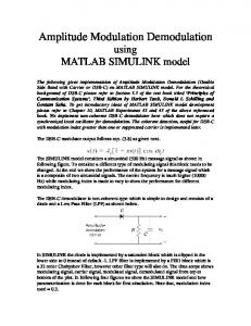
This section gives an application example to show how the equivalent stationary duration can be applied in the fitting of different amplitude modulation functions to a prescribed one. The intensity function specified in the Spanish version of Eurocode 8 Part 2 [11], as expressed in Eqs. (21) and (22), will be used as the reference function with α=0.05. The duration of the accelerograms must be consistent with the magnitude and other relevant features of the seismic event. According to the Spanish version of Eurocode 8 Part 1-1 [34], the duration of the stationary part of the accelerogram is correlated with the design ground acceleration (DGA), agd, in epicentral zones. Eurocode 8 gives the values of the minimum stationary duration for different values of agd, in the absence of site specific data. No indication is given in the abovementioned code of the exact definition of the “duration of the stationary part”. In principle, it could be considered to be the part of the accelerogram corresponding to the flat segment in the intensity function. If so, for a DGA of, for instance, agd=0.20g, which corresponds to a stationary duration of 15 s, the nominal duration of the earthquake would be Tgn=75 s and the total duration Tgt=105 s for α=0.05; these do not seem reasonable values for actual earthquakes. That is why the stationary duration mentioned in the Eurocode has been interpreted here as the equivalent stationary duration previously defined. In this way, the nominal and total durations of the reference intensity function would be shortened to Tgn=37.1 s and Tgt=58.0 s, respectively, for agd=0.20g. Four analytical intensity functions, amongst the ones previously reviewed, have been fitted to the reference Eurocode function for a moderate seismicity region with a DGA of agd=0.10g, which corresponds to a stationary duration of 10 s, i.e., Tgs=10 s. This function has a nominal duration of Tgn=24.7 s and a total duration of Tgt=34.6 s for α=0.05. The fitted functions are: the potential-constantexponential ICD function of Eq. (20) with m=2 (a=0.1103, Tgt=34.6 s); the exponential-exponential IPD function of Eq. (23) (a=0.1160, b=0.3216, Tgt=34.6 s); the potential-exponential IPD function of Eq. (24) with a generic m (a=0.1712, m=0.8492, Tgt=31.6 s); and the sinusoidal IPD function of Eq. (25) (m=2.4521, n=0.3565, Tgt=34.6 s). In the case of the ICD intensity function, the initial and final instants of the flat segment have been given equal values to those of the reference function, while the decreasing part has been fitted to give a value α=0.05 at the end of the earthquake (t=Tgt). In the case of the IPD intensity functions, the rise time tr has been taken to coincide with the middle time of the flat segment of the reference function, and the exponentially decreasing part has also been fitted with α=0.05. In the case of the sinusoidal function the nominal duration in which the function is defined, has been taken as Tgn=Tgt, with t1=0 and t2=Tgt.

1.2 EC-8

1.0

Potential-Constant-Exponential

Iag

0.8 0.6 0.4 0.2 0.0 0

5

10

15

20 t (s)

25

30

35

40

Figure 1. Eurocode 8 intensity function and fitted potential-constant-exponential ICD function.

Iag

1.2 1.0

EC-8

0.8

Exponential-Exponential

0.6 0.4 0.2 0.0 0

5

10

15

20

25

30

35

40

t (s)

Figure 2. Eurocode 8 intensity function and fitted exponential-exponential IPD function.

The results are shown in Figs. 1 to 4, where it can be observed the good fitting obtained when imposing the equality of the equivalent stationary duration to different amplitude modulation functions. The best fitting corresponds to the potential-constant-exponential and exponential-exponential functions, which are some of the most commonly used theoretical intensity functions. Worthy of mention is the fact that an identical or similar value of the total earthquake duration has been obtained in all the fitted intensity functions. This can be considered to be a proof of the coherency of the used mathematical constraints, as well as of the robustness of the new equivalent duration parameter. CONCLUSIONS

The equivalent stationary duration defined in this paper as the integral of the squared time-domain intensity function, has been shown to possess remarkable advantages over some other popular duration definitions such as bracketed or effective duration. One of the main advantages of the new earthquake duration definition is that it enables us to establish an equivalence criterion between different intensity functions. In this manner, once an equivalent duration is specified for a particular earthquake, almost any similar analytical or empirical amplitude modulation function can be used to simulate accelerograms that adequately represent the energy content of the original process. It is also a robust parameter that establishes a direct relation between the amplitude spectrum and the variance spectrum of the underlying stationary process, avoiding the necessity of using additional scaling factors to adjust the total variance of the process. 1.2 EC-8

1.0

Potential-Exponential

Iag

0.8 0.6 0.4 0.2 0.0 0

5

10

15

20

25

30

35

40

t (s)

Figure 3. Eurocode 8 intensity function and fitted potential-exponential IPD function.

1.2 EC-8

1.0

Sinusoidal

Iag

0.8 0.6 0.4 0.2 0.0 0

5

10

15

20

25

30

35

40

t (s)

Figure 4. Eurocode 8 intensity function and fitted sinusoidal IPD function.

ACKNOWLEDGEMENTS

The authors gratefully acknowledge the financial support provided by the Technical University of Valencia for carrying out this work, under Grant PPI-06-02/2928 of the Research Support Program. REFERENCES

1. 2. 3. 4. 5.

6. 7. 8.

9. 10. 11. 12.

Page CH. “Instantaneous power spectra.” Journal of Applied Physics, 1952; 23: 103-106. Priestley MB. “Evolutionary spectra and non-stationary processes.” Journal of the Royal Statistical Society, Series B, 1965; 27: 204-237. Mark WD. “Spectral analysis of the convolution and filtering of non-stationary stochastic processes.” Journal of Sound and Vibration, 1970; 11: 19-63. Liu SC. “Synthesis of stochastic representations of ground motions.” The Bell System Technical Journal, 1970; 49: 521-541. Polhemus NW, Cakmak AS. “Simulation of earthquake ground motions using autoregressive moving average (ARMA) models.” Earthquake Engineering and Structural Dynamics, 1981; 9: 343354. Carli F, Faravelli L. “A nonstationary seismological model for strong ground motions.” European Earthquake Engineering, 1990; IV(3): 29-42. Ólafsson, S. “The use of ARMA models in strong motion modelling.” Proceedings of the 10 th World Conference on Earthquake Engineering, Madrid, Spain, 1992; 2: 857-862. Faravelli L. “Modeling the seismic input for a stochastic dynamic structural problem.” Proceedings of the 5th International Conference on Application of Statistics and Probability in Soil and Structures, Vancouver, Canada, 1987; 230-237. Jennings PC, Housner GW, Tsai NC. “Simulated earthquake motions.” Report of the Earthquake Engineering Research Laboratory, California Institute of Technology, Pasadena, California, 1968. Amin M, Ang HS. “Non stationary stochastic model of earthquake motion.” Journal of the Engineering Mechanics Division, 1968; 94(EM2): 559-583. UNE-ENV 1998-2:1998. “Eurocode 8: Design provisions for earthquake resistance of structures Part 2: Bridges.” AENOR, Spanish official version of ENV 1998-2:1994, March 1998. Shinozuka M, Sato Y. “Simulation of nonstationary random process.” Journal of the Engineering Mechanics Division, 1967; 93(EM1): 11-40.

13. 14. 15.

16. 17. 18. 19. 20. 21.

22. 23. 24. 25. 26. 27. 28. 29.

30. 31.

32. 33. 34.

Bogdanoff JL, Goldberg JE, Bernard MC “Response of a simple structure to a random earthquaketype disturbance.” Bulletin of the Seismological Society of America, 1961; 51(2): 293-310. Saragoni GR, Hart C. “Simulation of artificial earthquakes.” Earthquake Engineering and Structural Dynamics, 1974; 2(3): 249-267. Tung ATY, Wang JN, Kiremidjian A, Kavazanjian E. “Statistical parameters of AM and PSD functions for the generation of site-specific strong ground motions.” Proceedings of the 10th World Conference on Earthquake Engineering, Madrid, Spain, 1992; 2: 867-872. Trifunac MD, Novikova EI. “State of the art review on strong motion duration.” Proceedings of the 10th European Conference on Earthquake Engineering, Vienna, Austria, 1994; 1: 131-140. Bommer JJ, Martínez-Pereira A. “The effective duration of earthquake strong motion.” Journal of Earthquake Engineering, 1999; 3: 127-172. Bolt BA. “Duration of strong ground motion.” Proceedings of the 5th World Conference on Earthquake Engineering, Rome, Italy, 1973; 1: 1304-1313. Ambraseys NN, Sarma SK. “The response of earth dams to strong earthquakes.” Geotechnique, 1967; 17: 181-213. Page RA, Boore DM, Joyner WB, Coulter HW. “Ground motion values for use in the seismic design of the trans-Alaska pipeline system.” US Geological Survey, Circular No. 672, 1972. McGuire RK, Barnhard TP. “The usefulness of ground motion duration in predicting the severity of seismic shaking.” Proceedings of the 2nd US National Conference on Earthquake Engineering, Stanford, CA, 1979; 713-722. Kawashima K, Aizawa K. “Bracketed and normalized durations of earthquake ground acceleration.” Earthquake Engineering and Structural Dynamics, 1989; 18: 1041-1051. Sarma SK, Casey BJ. “Duration of strong motion in earthquakes.” Proceedings of the 9th European Conference on Earthquake Engineering, Moscow, USSR, 1990; 10-A: 174-183. Arias A. “A measure of earthquake intensity.” Seismic Design of Nuclear Power Plants, RJ Hansen ed., MIT Press, Cambridge, MA, 1970; 438-483. Husid R, Medina H, Ríos J. “Análisis de terremotos norteamericanos y japoneses.” Revista del IDIEM, Santiago, Chile; 8. (in Spanish) Donovan NC. “Earthquake hazard for buildings.” Buildings Science Series, 1972; 46: 82-111. Trifunac MD, Brady AG. “A study on the duration of strong earthquake ground motion.” Bulletin of the Seismological Society of America, 1975; 65(3): 581-626. Trifunac MD, Westermo BD. “Duration of strong earthquake shaking.” Soil Dynamics and Earthquake Engineering, 1982; 2: 117-121. Novikova EI, Trifunac MD. “Duration of strong ground motion in terms of earthquake magnitude, epicentral distance, site conditions and site geometry.” Earthquake Engineering and Structural Dynamics, 1994; 23: 1023-1043. McCann MW, Shah HC. “Determining strong-motion duration of earthquakes.” Bulletin of the Seismological Society of America, 1979; 69: 1253-1265. Sabetta F. “Analisi di quattro definizioni di durata applicate ad accelerogrammi relativi a terremoti italiani.” Italian Agency for New Technologies, Energy and Environment, Rome, Italy, 1983. (in Italian) Vanmarcke EH, Lai S-SP. “Strong motion duration and rms amplitude of earthquake ground motion.” Bulletin of the Seismological Society of America, 1980; 70(4): 1293-1307. Carli F. “Smooth frequency modulating functions for strong ground motions.” Proceedings of the 10th European Conference on Earthquake Engineering, Vienna, Austria, 1994; 155-160. UNE-ENV 1998-1-1:1998. “Eurocode 8: Design provisions for earthquake resistance of structures. Part 1-1: General rules, seismic actions and general requirements for structures.” AENOR, Spanish official version of ENV 1998-1-1:1994, March 1998.