ERROR ESTIMATES FOR THE ANOVA METHOD WITH ...

ERROR ESTIMATES FOR THE ANOVA METHOD WITH POLYNOMIAL CHAOS INTERPOLATION: TENSOR PRODUCT FUNCTIONS ∗ ZHONGQIANG ZHANG, MINSEOK CHOI AND GEORGE EM KARNIADAKIS

†

Abstract. We focus on the analysis of variance (ANOVA) method for high dimensional function approximation using Jacobi-polynomial chaos to represent the terms of the expansion. First, we develop a weight theory inspired by quasi-Monte Carlo theory to identify which functions have low effective dimension using the ANOVA expansion in different norms. We then present estimates for the truncation error in the ANOVA expansion and for the interpolation error using multi-element polynomial chaos in the weighted Korobov spaces over the unit hypercube. We consider both the standard ANOVA expansion using the Lebesgue measure and the anchored ANOVA expansion using the Dirac measure. The optimality of different sets of anchor points is also examined through numerical examples. Key words. anchored ANOVA, effective dimension, weights, anchor points, integration error, truncation error

Notation. c, ck : points in one dimension. c: point in high dimension. ck : optimal anchor points in different norms. Ds : mean effective dimension. ds : effective dimension. f{i} : i-th first-order terms in ANOVA decomposition. f (i) : function of the i–th dimension of a high dimensional tensor product function. Gi : i-th GENZ function. I(·): integration of the function “ · ” over [0, 1]N or [0, 1]. IN,ν f : truncated ANOVA expansion with only terms of order lower than ν + 1. IN,ν,µ f : multi-element approximation of IN,ν f with tensor-products of µ-th order polynomials in each element. L2 (·): space of square integrable functions over the domain “ · ”; the domain will be dropped if no confusion occurs. L∞ (·): space of essentially bounded functions over the domain “ · ”; the domain will be dropped as above. N : dimension of a high dimensional function. wk : sampled points from a uniform distribution on [0, 1]. µ: polynomial order. ν: truncation dimension. τk : mean of the function f (k) ; λ2k : variance of the function f (k) . σ 2 (·): variance of the function “ · ”. 1. Introduction. Functional ANOVA refers to the decomposition of an N dimensional function f as follows [9]: f (x1 , x2 , · · · , xN ) = fφ +

N X

j1 =1

f{j1 } (xj1 ) +

N X

j1 21 and C2 depends only on r. See Ma [12] and Li [11] for proofs. By (3.2), for fixed S, we have X

kfS − IS,ν,µ fS kL2 ([0,1]|S| ) ≤ C2 hk 2−k µ−rn ∂xrnn fS L2 ([0,1]|S| ) , n∈S

where rn = r is the regularity index of fS as a function of xn . Thus, taking γn = γ gives 1

kfS − IS,ν,µ fS kL2 ([0,1]|S| ) ≤ C2 |S| 2 (γ

|S| 2

hk 2−k µ−r ) kfS kK r ([0,1])⊗|S| . γ

(3.3) 1

1

Here we have utilized the inequality of (a1 + a2 + · · · + an ) ≤ n 2 (a21 + a22 + · · · + a2n ) 2 for real numbers. Following (3.3), we then have X kIN,ν f − IN,ν,µ f kL2 ([0,1]N ) ≤ kfS − IS,ν,µ fS kL2 ([0,1]|S| ) S⊆{1,2,··· ,N }

1≤|S|≤ν

≤

1

X

C2 |S| 2 hk 2−k µ−r γ

|S| 2

kfS kK r ([0,1])⊗|S| γ

∅6=S⊆{1,··· ,N }

|S|≤ν 1

≤ C2 ν 2 hk 2−k µ−r

X

γ

|S| 2

kfS kKγr ([0,1])⊗|S| .

∅6=S⊆{1,··· ,N }

|S|≤ν

This ends the proof. Remark 3.5. Taking h = 1 in Theorem 3.4 gives the following estimate 1

kIN,ν f − IN,ν,µ f kL2 ([0,1]N ) ≤ Cν 2 2−k µ−r

X

γ

|S| 2

kfS kK r ([0,1])⊗|S| . γ

∅6=S⊂{1,··· ,N }

|S|≤ν

It is worth mentioning that the factor in front of µ−r can be very large ifPN is large.
ν Also large ν can lead to large values of the summation since there are k=1 Nk ≈
N ν N ν terms even if ν < 2 . And again, if the weights are not small, then the norm of fS can be very large; the norms can be small and grow relatively slowly with ν when the weights are much smaller than 1. Remark 3.6. Section 5 of [23] gives an example of functions in Korobov spaces in
−1 applications. The function is of tensor-product, f (x) = ⊗N (xk ) , where k=1 exp ak Φ Rx 1 ak = O(N − 2 ), k = 1, 2, · · · , N, and Φ−1 (x) is the inverse of Φ(x) = √12π −∞ 2

exp(− t2 ) dt. It can be readily checked that γk =

λ2k exp(a2k )(exp(a2k ) − 1) = exp(a2k ) − 1, = 2 τk (exp( 12 a2k ))2 14

k = 1, 2 · · · , N,

and according to (2.7), Ds = O(1). This implies that the problem is of low effective dimension. These weights decay fast, thus contributing to the fast convergence rate in the approximation. Remark 3.7 (Multi-element interpolation error for piecewise continuous functions). For piecewise continuous functions, the interpolation error can be bounded as X |S| 1 h γ 2 kfS kKγr ([0,1]⊗|S| ) , kIN,ν f − IN,ν,µ f kL2 ([0,1]N ) ≤ Cν 2 ( )µ+1 µ−r 2 S⊂{1,2,··· ,N }

|S|≤ν

where h is the length of one edge in an element, ν the truncation dimension, µ the polynomial order and the constant C depends only on r. 4. Error estimates of (Lebesgue) ANOVA for continuous functions. The results for the standard ANOVA with the Lebesgue measure are very similar to the results for the anchored ANOVA. We present them here without any proofs as the proofs are similar to those in Section 3. Here we will adopt another weighted Korobov space Hγr ([0, 1]). For an integer r, the space is equipped with the following inner product ! r−1 X ≺ f, g ≻Hγr ([0,1]) = I(f )I(g) + γ −1 I(∂xk f )I(∂xk g) + I(∂xr f ∂xr g) k=1

1 2

and the norm kf kHγr ([0,1]) =≺ f, f ≻H r ([0,1]) . Again using the Hilbert space interγ polation [1], such a space with non-integer r can be defined. The product space Hγr ([0, 1])⊗N := Hγr ([0, 1]) × · · · × Hγr ([0, 1]) (N times) is defined in the same way of defining Kγr ([0, 1])⊗N in Section 3. Theorem 4.1 (Truncation error). Assume that the tensor product function f belongs to Hγr ([0, 1])⊗N . Then the truncation error of the standard ANOVA expansion can be bounded as X |S|−ν−1 ν+1 kf − IN,ν f kL2 ([0,1]N ) ≤ (Cγ2−2r ) 2 kfS kHγr ([0,1])⊗|S| , (Cγ2−2r ) 2 S⊂{1,2,··· ,N }

|S|≥ν+1

where the constant C is decreasing with r. The proof of this theorem is similar to that of Theorem 3.1. One first finds a complete orthogonal basis both in L2 ([0, 1])∩{f : I(f ) = 0} and H1r ([0, 1])∩{f : I(f ) = 0} by investigating the eigenvalue problem of the Rayleigh quotient

kf k2L2 ([0,1])

kf k2H r ([0,1])

(see Ap-

1

pendix for the definition of the eigenvalue problem) and following the proof of Theorem 3.1. The following theorem can be proved in the same fashion as in Theorem 3.4. Theorem 4.2 (Interpolation error). Assume that the tensor product function f lies in Hγr ([0, 1])⊗N , where r > 21 . Then the interpolation error of the standard ANOVA expansion can be bounded as X |S| 1 kIN,ν f − IN,ν,µ f kL2 ([0,1]N ) ≤ Cν 2 2−k hk µ−r γ 2 kfS kH r ([0,1])⊗|S| , γ

S⊂{1,2,··· ,N }

|S|≤ν

where k = min (r, µ + 1), IN,ν,µ f is defined as in Section 3.2 and the constant C depends solely on r. 15

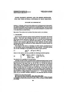
5. Numerical results. Here we provide numerical results, which verify the aforementioned theorems and show the effectiveness of the anchored ANOVA expansion and its dependence on different anchor points. 5.1. Verification of the error estimates. We compute the truncation error |4xk −2|+ak , in the standard ANOVA expansion of the Sobol’s function f (x) = ⊗N k=1 1+ak where we compute the error for ak = 1, k and k 2 with N = 10. In Figure 5.1 we show numerical results for ak = k and N = 10 along with the error estimates that demonstrate good agreement. For ak = 1 and k 2 , we have similar trends for the decay of error, and in particular we observe that larger ak (hence, smaller weights) will lead to faster error decay.

Fig. 5.1. Truncation and interpolation error in L2 : Comparison of numerical results against error estimates from Theorems 4.1 and 4.2. Left: Truncation error; Right: Interpolation error.

Compared to Figure 2.1, there is no sudden drop in Figure 5.1 (left) since the 1 weights γkA = 3(1+k) 2 are basically larger than those of G5 in the Example 2.2 and decay slowly; this points to the importance of higher order terms in the standard ANOVA expansion. In Figure 5.1 (right), we note that small µ may not admit good approximations of the ANOVA terms. 5.2. Genz function G4 [8]. Consider a ten-dimensional Genz function G4 = P10 exp(− i=1 x2i ), where the relative integration error and truncation error are considered. In this case, only second-order terms are required for obtaining small ν 0 1 2 3 4 5 6

ǫν,c1 (G4 ) 2.8111 e-2 5.5920 e-3 6.3516 e-4 4.6657 e-5 2.3331 e-6 8.0681 e-8 1.9081 e-9

ǫν,c2 (G4 ) 3.1577 e-2 1.0985 e-2 2.4652 e-3 3.7620 e-4 4.0082 e-5 2.9961 e-6 1.5455 e-7

ǫν,c4 (G4 ) 6.9005 e-6 3.9702 e-10 1.4093 e-14 2.7825 e-15 9.6520 e-15 3.6533 e-14 3.4521 e-14

ǫν,c5 (G4 ) 5.4637 e-2 1.8717 e-2 3.5770 e-3 4.3819 e-4 3.6379 e-5 2.0833 e-6 8.1459 e-8

Table 5.1 Relative integration errors for G4 using different anchor points: N = 10.

integration error in Table 5.1. For the truncation error, shown in Table 5.2, more terms are required to reach a level of 10−3 , and the convergence is rather slow. Note 16

ν 0 1 2 3 4 5 6 7 8 9

εν,c1 (G4 ) 6.1149 e-2 3.6243 e-2 1.6569 e-2 6.0440 e-3 1.7925 e-3 4.3473 e-4 8.5654 e-5 1.3402 e-5 1.5799 e-6 1.2184 e-7

εν,c2 (G4 ) 6.2818 e-2 3.9884 e-2 1.9881 e-2 7.9242 e-3 2.5497 e-3 6.6163 e-4 1.3662 e-4 2.1745 e-5 2.4900 e-6 1.7163 e-7

εν,c3 (G4 ) 5.4305 e-2 2.8965 e-2 1.2297 e-2 4.2887 e-3 1.2472 e-3 3.0346 e-4 6.1292 e-5 1.0045 e-5 1.2688 e-6 1.0819 e-7

εν,c4 (G4 ) 5.4305 e-2 2.8965 e-2 1.2297 e-2 4.2887 e-3 1.2472 e-3 3.0346 e-4 6.1292 e-5 1.0045 e-5 1.2688 e-6 1.0754 e-7

εν,c5 (G4 ) 7.7034 e-2 5.3008 e-2 2.6415 e-2 1.0098 e-2 3.0503 e-3 7.3564 e-4 1.4083 e-4 2.0877 e-5 2.2590 e-6 1.5257 e-7

Table 5.2 ‚ ‚ Truncation error ‚G4 − IN,ν (G4 )‚L2 versus truncation dimension ν using different anchor points: N = 10.

that for this example, the sparse grid method of Smolyak [17] does not work well either. 5.3. Genz function G5 [8]. Here we address the errors in different norms using different anchor points. Recall that c1 is the centered point and c2 , c4 and c5 are defined exactly as in Example 2.9. For these four different choices of anchor points, we test two cases: i) relative error of numerical integration using the anchored ANOVA expansion and ii) approximation error using the anchored ANOVA expansion in different norms, see Figure 5.2. In both cases c4 gives the best approximation followed by c5 . Observe that for this example c4 among the four anchor points gives the best approximation to the function with respect to the L1 , L2 and L∞ -norms although the theorems in Section 2 imply that different measures will lead to different “optimal” points. We have also verified numerically that the numerical integration error is bounded by the approximation error with respect to L1 and L∞ -norms as shown in Figure 5.3. For different choices of anchor points, the integration error is bounded by the approximation error between the function and its anchored ANOVA truncation with respect to the L1 -norm that is bounded by the approximation error with respect to the L∞ -norm. In addition to the above tests, we have also investigated the errors of the Genz functions G2 [8] with the same ci and wi as in Example 2.2; similar results were obtained (not shown here for brevity). 6. Summary. We considered the truncation of the ANOVA expansion for high dimensional tensor-product functions. We have defined different sets of weights that reflect the importance of each dimension. Based on these weights, we find that only those functions with small weights (smaller than 1) can admit low effective dimension in the standard ANOVA expansion. High regularity of a function would not necessarily lead to a smaller truncation error; instead only the functions with smaller weights have smaller truncation error. For the anchored ANOVA expansion, we proposed new anchor points, which minimize the weights in different norms to improve the truncation error. The optimality of different sets of anchor points is examined through numerical examples in measure of the relative integration error and the truncation error. For the L2 -truncation error, it seems that the choice of anchor points should be such that the target function at 17

Fig. 5.2. Testing Genz function G5 using different anchor points in different measure. Top left: relative integration error; Top right: relative error in the L1 -norm; Lower left: relative error in the L2 -norm; Lower right: relative error in the L∞ -norm.

the point has a value close to its mean. Numerical tests show the superiority of the anchor point c4 , which minimizes the weights with respect to numerical integration, compared to other anchor points. We also derived rigorous error estimates for the truncated ANOVA expansion, as well as estimates for representing the terms in truncated ANOVA expansion with multi-element methods. These estimates show that the truncated ANOVA expansion converges in terms of the weights and smoothness; the multi-element method converges to the truncated ANOVA expansion and thus it converges fast to the ANOVA expansion if the weights are small.

7. Appendix: Detailed proofs.

18

Fig. 5.3. Verification of the relationships between errors in different measures.

7.1. Proof of Theorem 2.5. By the anchored ANOVA expansion and the triangle inequality, we have QN kf − IN,˜ν f kL∞ k=1 f (k) (ck ) kf − IN,˜ν f kL∞ = QN (k) (ck ) kf kL∞ kf kL∞ k=1 f

(k)

PN P Q (k) Q

− f (k) (ck ) L∞ N (ck ) m=˜ ν +1 |S|=m k∈S f k=1 f ≤ QN (k) kf kL∞ (ck ) k=1 f N (k) N Y X X Y f (ck )

γk∞ ( ≤

f (k) ∞ ), m=˜ ν +1 |S|=m k∈S

k=1

L

where we used the definition of weights (2.9). Then the assumption with the above inequality yields the desired error estimate. The following will complete the proof of how to minimize the weights. Suppose that f (k) (xk ) does not change sign over the interval [0, 1]. Without loss of generality, let f (k) (xk ) > 0. Denote the maximum and the minimum of f (k) (xk ) by Mk and mk , respectively, and assume that f (k) (ck ) = αk Mk + (1 − αk )mk , where

(k) (k)

αk ∈ [0, 1]. Then f − f (ck ) L∞ = (Mk − mk ) max(1 − αk , αk ), and the weight

(k)

f − f (k) (ck ) ∞ (Mk − mk ) max(1 − αk , αk ) ∞ L γk = = . f (k) (ck ) αMk + (1 − αk )mk 19

max(1−αk ,αk ) Note that the minimum of the function g(αk ) = (1−mαkk)+(1−α can be only k )mk mk 1 attained at αk = 2 , where αk ∈ [0, 1], mk = Mk ∈ (0, 1). This ends the proof. We note that N N N (k) N Y Y Y

Y f (ck )

αk (1 − mk ) + mk max(2α , 1)(1 − m ) + m − = ( (1 + γk ) − 1) k k k

f (k) ∞ L k=1 k=1 k=1 k=1

attains its minimum at ( 12 , 21 , · · · , 12 ). Since smaller weights lead to smaller 1 − pν˜ , we have then a tighter error estimate (2.10).

7.2. Proof of Theorem 2.7. The inequality (2.12) can be readily obtained as in the proof of Theorem 2.5. (k) For simplicity, we denote αk = ff (k)(ck ) . To minimize the weights (2.11), αk has k kL2

(k)

f 2 L to be , since the quadratic function of α1k , τk 2 (γkL )2

2

f (k) τk 1 1

+ 1, − 1 = (k) = 2 −2

(k)

αk αk f L2 f (ck ) L2

(k)

f 2 L attains its minimum at αk = , for k = 1, 2, · · · , N . τk

7.3. Proof of Lemma 3.2. Here we adopt the methodology in [26] to prove the lemma. We will prove the lemma when r is an integer. When r is not an integer, we may apply the Hilbert space interpolation theory for K1r ([0, 1]). Define the eigenvalues of the Rayleigh quotient RK (f ) = K1r ([0, 1])

λn = inf

sup hf,ψi iK r ([0,1]) =0, 1≤i≤n−1 1 kf k2K r ([0,1]) =1 1

r ([0,1]) f ∈K1

kf k2K r ([0,1]) =1

kf k2K r ([0,1])

, for f ∈

1

as follows: for n ≥ 2,

with λ1 = inf sup

kf k2L2 ([0,1])

2

kf kL2 ([0,1])

2

kf kL2 ([0,1]) and ψi are the corresponding eigenfunctions

1

to λi with kψi kK r ([0,1]) = 1. 1 First, this eigenvalue problem is well-defined (see pp. 45, [26]) as hf, f iK1r ([0,1]) is positive definite and RK (f ) is bounded from above. In fact, for f ∈ K1r ([0, 1]) kf k2 2

Rk (f ) ≤ Cl−1 kf k2L r([0,1]) ≤ Cl−1 according to the following fact that there exist positive H ([0,1])

constants Cl and Cu independent of r and f such that 2

2

2

Cl kf kH r ([0,1]) ≤ kf kK r ([0,1]) ≤ Cu kf kH r ([0,1]) . 1

(7.1)

Pr 1 Here the Hilbert space H r ([0, 1]) has the norm kf kH r ([0,1]) = ( k=0 I((∂xk f )2 )) 2 . We will prove this fact shortly. 2 2 Second, kf kL2 ([0,1]) is completely continuous with respect to kf kK r ([0,1]) by defi1 nition (see pp. 50, [26]). This can be seen from the following. By Poincare-Friedrich inequality [26], for any ǫ > 0, there exists a finite set of linear functionals l1 , l2 , · · · , lk 20

such that for f with f (c) = 0, li (f ) = 0, i = 1, · · · , k implies that R1 ǫ 0 (∂x f )2 dx and hence that, by (7.1), Z

1

2

f dx ≤ ǫ

0

Z

1

0

2

R1 0

f 2 dx ≤

2

(∂x f )2 dx ≤ ǫ kf kH r ([0,1]) ≤ Cl−1 ǫ kf kK r ([0,1]) . 1

Since the two forms (·, ·)L2 ([0,1]) and h·, ·iK1r ([0,1]) are positive definite, according to Theorem 3.1, pp. 52, [26], the eigenfunctions corresponding to the eigenvalues of the Rayleigh quotient RK (f ) actually form a complete orthogonal basis not only in L2 ([0, 1]) but in K1r ([0, 1]). By (7.1) and the second monotonicity principle (Theorem 8.1, pp. 62, [26]), λn ∈ 2 kf kL2 ([0,1]) [Cu−1 βn , Cl−1 βn ] where βn are eigenvalues of the Rayleigh quotient . Note 2 kf kH r ([0,1]) that the βn are of order n−2r . Actually, a complete orthogonal basis both in L2 ([0, 1]) ∞ and H r ([0, 1]) is {cos(nπx)}n=0 . Thus βn = (nπ)−2r and λn ≤ C1 n−2r , where C1 decreases with r. At last, it can be readily checked that the first eigenvalue λ1 = 1 and the corresponding eigenfunction is the constant 1. Recall that K1r ([0, 1]) can be decomposed r as span {1} ⊕ K1,0 ([0, 1]). We then reach the conclusion if (7.1) is true. Now we verify (7.1). By the Sobolev embedding inequality, we have kf kL∞ ≤ Cs kf kH 1 ([0,1]) . Since |g(c)| ≤ kgkL∞ for any g ∈ K1r ([0, 1]), this leads to r−1 X

[∂xi f (c)]2 +

i=1

Z

0

1

[∂xr f (x)]2 dx ≤

1 2 C 2 s

2

Z

1

0

r

X 1 (∂x f )2 dx + ( Cs2 + 1) 2

k=2

Z

0

1

(∂xk f )2 dx.

2

This proves that kf kK r ([0,1]) ≤ Cu kf kH r ([0,1]) , where Cu = Cs2 + 1. The inequality 2

2

1

Cl kf kH r ([0,1]) ≤ kf kK r ([0,1]) can be seen from the basic inequality, for any c ∈ [0, 1], 1 Z 1 Z 2 1 2 2 f (x) dx ≤ 2f (c)+ [∂x f (x)]2 dx. Applying repeatedly this inequality for ∂xk f 3 0 0 (k = 1, · · · , r) and summing them up, we have, with Cl = 61 , 2

kf kH r ([0,1]) =

Z

0

1

f 2 (x)dx +

r−1 Z X

k=1

1

0

2

[∂xk f (x)]2 dx ≤ Cl−1 kf kK r ([0,1]) . 1

REFERENCES [1] R. Adams, Sobolev spaces, Academic Press, New York, 1975. [2] M. Bieri and C. Schwab, Sparse high order FEM for elliptic sPDEs, Comput. Methods Appl. Mech. Engrg., (198) 2009, pp. 1149–1170. [3] R. E. Caflisch, W. Morokoff, and A. Owen, Valuation of mortgage-backed securities using brownian bridges to reduce effective dimension, J. Comput. Finance, 1 (1997), pp. 27–46. [4] Y. Cao, Z. Chen, and M. Gunzbuger. ANOVA expansions and efficient sampling methods for parameter dependent nonlinear PDEs, Int. J. Numer. Anal. Model., 6(2009), pp. 256–273. [5] J. Dick, I. H. Sloan, X. Wang, and H. Wozniakowski, Liberating the weights, J. Complexity, 20 (2004), pp. 593–623. [6] J. Foo and G. E. Karniadakis, Multi-element probabilistic collocation method in high dimensions, J. Comput. Phys., 229 (2010), pp. 1536–1557. [7] J. Foo, X. Wan, and G. E. Karniadakis, The multi-element probabilistic collocation method (me-pcm): Error analysis and applications, J. Comput. Phys., 227 (2008), pp. 9572–9595. 21

[8] A. Genz, A package for testing multiple integration subroutines,, in Numerical Integration: Recent Developments, Software and Applications, P. Keast and G. Fairweather, eds., Reidel, 1987, pp. 337–340. [9] M. Griebel, Sparse grids and related approximation schemes for higher dimensional problems, in Foundations of Computational Mathematics (FoCM05), Santander, L. Pardo, A. Pinkus, E. Suli, and M. Todd, eds., Cambridge University Press, 2006, pp. 106–161. [10] M, Griebel and M, Holtz, Dimension-wise integration of high-dimensional functions with applications to finance, INS Preprint No. 0809, University of Bonn, Germany, Jan. 2009. [11] H. Y. Li, Super spectral viscosity methods for nonlinear conservation Laws, Chebyshev collocation methods and their applications, PhD thesis, Shanghai University, 2001. [12] H. P. Ma, Chebyshev-Legendre spectral viscosity method for nonlinear conservation laws, SIAM J. Numer. Anal., 35 (1998), pp. 869–892. [13] A. B. Owen, Necessity of low effective dimension, manuscript, Oct. 2002. , The dimension distribution and quadrature test functions, Statist. Sinica, 13 (2003), [14] pp. 1–17. [15] A. Papageorgiou, Sufficient conditions for fast quasi-Monte carlo convergence, J. Complexity, 19 (2003), pp. 332 – 351. [16] S. H. Paskov and J. F. Traub, Faster valuation of financial derivatives, J. Portfol. Manage., 22 (1995), pp. 113–120. [17] K. Petras, On the Smolyak cubature error for analytic functions, Advances in Computational Mathematics, 12 (2000), pp. 71–93. [18] I. H. Sloan and H. Wozniakowski, When are Quasi-Monte Carlo algorithms efficient for high dimensional integrals?, J. Complexity, 14 (1998), pp. 1–33. [19] S. Tezuka, Quasi-Monte Carlo: discrepancy between theory and practice, in Monte Carlo and Quasi-Monte Carlo Methods 2000, K. T. Fang, F. J. Hickernell, and H. Niederreiter, eds., Springer, Berlin, 2002, pp. 124–140. [20] R. A. Todor and C. Schwab, Convergence rates for sparse chaos approximations of elliptic problems with stochastic coefficients, IMA J. Numer. Anal., 27 (2007), pp. 232–261. [21] X. Wan and G. E. Karniadakis, An adaptive multi-element generalized polynomial chaos method for stochastic differential equations, J. Comput. Phys., 209 (2005), pp. 617 – 642. [22] X. Wang and K.-T. Fang, The effective dimension and quasi-Monte Carlo integration, J. Complexity, 19 (2003), pp. 101–124. [23] X. Wang and I. H. Sloan, Why are high-dimensional finance problems often of low effective dimension?, SIAM J. Sci. Comput., 27 (2005), pp. 159–183. [24] X. Wang and I. H. Sloan, Efficient weighted lattice rules with applications to finance, SIAM J. Sci. Comput., 28 (2006), pp. 728–750. [25] X. Wang, Strong tractability of multivariate integration using quasi-Monte Carlo algorithms, Math. Comput., 72 (2003), pp. 823–838. [26] H. F. Weinberger, Variational Methods for eigenvalue approximation, vol. 15 of Regional Conference Series in Applied Mathematics, SIAM, Philadelphia, Pennsylvania, 1974. [27] X. Yang, M. Choi, G. Lin, and G. E. Karniadakis, Adaptive anova decomposition of stochastic incompressible and compressible flows, Journal of Computational Physics, (2011), In press.

22