Science & Technology Corporation. Hampton ... evaluated with airline actions in Airspace Flow Programs. ...... opmen
Ninth USA/Europe Air Traffic Management Research and Development Seminar (ATM2011)
Evaluating Delay Cost Functions with Airline Actions in Airspace Flow Programs Michael Bloem
Haiyun Huang∗
NASA Ames Research Center Moffett Field, CA, USA
[email protected]
Science & Technology Corporation Hampton, VA, USA and Delft University of Technology Delft, the Netherlands
[email protected]
Abstract— Air traffic management research and simulation use delay cost functions that attempt to quantify the cost of delay to airlines. Seventeen delay cost functions from previous research are evaluated with airline actions in Airspace Flow Programs. Airline actions from 34 days in the summer of 2006 were used to compute four metrics designed to quantify the consistency of the airline actions with each of the cost functions. Two of these metrics compare the cost of airline actions to the cost of the default first-scheduledfirst-served actions. These metrics identify delay cost functions in which costs increase in discrete steps as delay increases as most consistent with airline actions. The other two metrics compare the cost of the airline actions to the minimum costs. These metrics identify delay costs that are proportional to the length of delay but with larger proportionality constants for flights bound for hub airports as most consistent with airline actions. Keywords— Delay; Metrics; Airline Behavior Modeling; Collaborative Decision Making; Air Traffic Flow Management Slots; Airspace Flow Programs
N OMENCLATURE (F , S, M) α β(tf , d) δ η(ef , d) γ(f ) γ ′ (f, af ) ˆ 2) L(σ ρ(d) σ 2⋆ ˜ FSFS R ˜ Rmin ε af ∗ Supported
Set of corresponding sets of flights, sets of slots, and matchings Weighting parameter Time-of-Day Delay multiplier Length of slot time window in minutes Monetary Delay multiplier Connection Delay multiplier Airline Connection Delay multiplier Approximate log-likelihood when the variance is σ 2 and the mean is assumed 0 Step delay cost Estimate of the additive cost noise variance Median of FSFS ratios Median of minimum ratios Additive cost noise Airline operating flight f by STC/STIEP/IRAD 6700-112
c(f, d)
Delay cost function for flight f and d minutes of delay d Delay in minutes d(f, s) Delay in minutes resulting from assigning flight f to slot s ef Aircraft type used for flight f F Set of flights f A flight I Improvement frequency J(F, S, M, c) The cost of matching the set of flights F to the set of slots S as specified by matching M when using cost function c J ⋆ (F, S, c) Minimum cost for a perfect matching of the flights F to the slots S when the cost function is c M A matching of flights to slots n Number of flights and slots pf Number of passengers on flight f RFSFS The FSFS ratio Rmin The minimum ratio S Set of slots s A slot tf Scheduled time of arrival for flight f ts Slot time I.
I NTRODUCTION
The cost of delaying a flight differs from flight to flight. This cost can be most accurately estimated by the airlines, but unfortunately airlines are reluctant to reveal their costs because doing so could be advantageous to their competitors. Having an accurate understanding of airline costs is important in air traffic management research. Airline cost functions impact the design of air traffic management concepts, help determine the value of new concepts, and can form the basis of airline behavior models used in simulations. Without the benefit of knowing actual airline delay costs, researchers must infer these costs. Only one effort has been made to tune and validate delay cost functions with records of airline actions. In her disserta-
tion [1], Xiong used airline flight cancellation and slot usage data from Ground Delay Programs to tune parameters in discrete choice models of airline behavior. Discrete choice models assign a probability to every possible choice an airline has based on the cost of each choice. Xiong’s research revealed many characteristics of airline delay costs, but there are some limitations of her work. Discrete choice models cannot easily handle cases with many discrete choices, preventing the use of some of the available data. More importantly, Xiong did not study any “separable” delay cost models. Separable delay cost models use a flight delay cost function to compute the cost of delaying each flight and assume that the total airline cost is the sum of the individual flight delay costs. While there are exceptions [2–8], most research uses a separable delay cost model [9–18]. Some airline decision support tools are also based on separable delay cost models [19–21]. Furthermore, Xiong’s use of Ground Delay Program data limited her ability to investigate the difference in the cost of delay for hub-bound flights and other flights. Finally, while Xiong studied linear models with dataintensive variables related to airline revenues, her work did not consider some simple variables from previous research and airline decision-support tools, such as those in [20, 22–24]. The goal of this research is to determine the degree to which delay cost functions proposed for separable delay cost models are consistent with how airlines assign flights to slots in Airspace Flow Programs. None of these delay cost functions have been validated with airline actions. The inability of discrete choice models to handle cases with many choices would prevent the use of more than half of the available data for some airlines, so a new approach for validating cost functions is needed. Four new metrics are proposed for evaluating the extent to which cost functions are consistent with airline actions in Airspace Flow Programs. Two of the four metrics compare the costs incurred by airlines to the costs of default actions, while the other two compare to the minimum costs. One metric adds a noise term to delay cost functions to account for unobserved aspects of airline costs and then estimates the parameters of the noise with airline action data. The remainder of this paper is structured as follows. Section II contains background information about Airspace Flow Programs. The model, metrics, and data used to evaluate cost functions are presented in Section III. Results are discussed in Section IV. The paper finishes with proposals for future work in Section V and conclusions in Section VI. II.
BACKGROUND
Airspace Flow Programs (AFPs) are a mechanism used by the Federal Aviation Administration (FAA) in the United States to assign departure delays to aircraft when demand for a region of airspace known as a “Flow Constrained Area” (FCA) exceeds capacity. This mechanism is based on the concept of slots. A slot is the right to fly into the FCA in a specified period of time. The FAA enforces slot ownership rights by assigning departure times to flights bound for an FCA so that each flight arrives at the FCA approximately at the time of the slot to which it is assigned. During AFPs, slots are allocated to airlines with
an algorithm referred to as “ration by schedule” (RBS) that is based on a first-scheduled-first-served (FSFS) principle. By default, each airline’s flights are assigned to their allocated slots in a FSFS manner, but they can adjust this assignment as they see fit. Large airlines alter the assignment of their flights to their slots in AFPs thousands of times each year. III.
M ETHOD
A.
Airline Behavior Model Airlines have tools and procedures that allow them to make acceptable decisions during an AFP, but the problem they face during an AFP is complicated and difficult for researchers to model [25]. There are many possible ways for an airline to assign their flights to their slots. A flight can be canceled or routed out of the relevant FCA. The assignment of flights to slots is not just a one-time decision but can be changed repeatedly during the AFP. Uncertain factors impact the airline, such as if and how the FAA will alter the AFP parameters and when the AFP will end. Cancelations by other airlines can impact an airline’s allocation of slots. Furthermore, the impact of delaying each flight is difficult to compute because passenger, luggage, crew, and aircraft connections mean that delaying one flight may impact several other flights. Mechanical or crew “time-out” issues can arise and further complicate matters. It is not obvious to researchers how airlines consider all of these factors when making decisions. To make this problem tractable, a separable delay cost model will be assumed. More specifically, it is assumed that airlines attempt to minimize the sum of the delay costs associated with assigning each flight to each slot. This model assumes that airlines ignore the dynamic nature of the AFP, uncertainties, the possibility of canceling flights or routing them out of the FCA, and the behavior of other airlines, except when the flight delay cost function attempts to include such issues. More sophisticated models and solution methods have been developed that consider the possibility of canceling flights, non-separable cost functions, and other issues [3–7, 19]. These techniques may be more accurate, but the separable delay cost model allows for computationally simple evaluations of delay cost functions with AFP data. If airlines minimize a separable delay cost, then the problem faced by airlines when assigning flights to slots is well-known and referred to as the “minimum cost perfect matching” or “assignment” problem. Given a set of flights and slots, a “matching” is a set of connections between flights and slots such that flights are matched to only one slot and vice versa. A “perfect matching” is any matching in which no flight or slot is left unmatched. Several algorithms can solve this problem efficiently, even for cases where there are hundreds or thousands of flights and slots. This is not necessarily the case for the more sophisticated problem models. B.
Notation Before defining the four metrics used to evaluate the degree to which a delay cost function is consistent with historical
assignments of flights to slots in AFPs, some notation will be introduced. Let F be the set of flights belonging to an airline in a matching, and let S be the airline’s slots in the matching. The number of flights and slots is n. Associated with each flight f ∈ F is a scheduled time of arrival at the constrained resource tf and associated with each slot s ∈ S is a time ts and a time window [ts , ts + δ] for some δ ≥ 0. A flight f can only be assigned to a slot s if tf ≤ ts + δ. The cost of assigning a flight f to a slot s is given by the cost function under consideration, which is a function of f and the delay associated with assigning f to s. There are historical assignments of flights to slots where tf > ts , so delay is computed as d(f, s) = max{0, ts − tf }. This information makes up the data for the minimum cost perfect matching problem assumed to be solved by the airline. The set of historical matchings of flights and slots by an airline is denoted by (F , S, M). An element (F, S, M ) ∈ (F , S, M) contains the set of flights F and set of slots S associated with a matching M selected by an airline. The matching M is a perfect matching that assigns each f ∈ F to exactly one s ∈ S. It is a square binary matrix with an entry for each possible assignment of a flight to a slot. Element Mij is 1 if fi is assigned to slot sj and is 0 otherwise. For a cost function ck , the cost of a matching is X
J(F, S, M, ck ) =
Some example matchings are shown in Fig. 2. Fig. (a) is the default FSFS matching (M FSFS ), Fig. (b) is the airline-selected matching (M ), Fig. (c) is a minimum cost perfect matching for some cost function A, and Fig. (d) is a minimum cost perfect matching for some cost function B.Fig. 3 shows example cost values incurred by these matchings.
(a) FSFS matching (M FSFS )
(b) Airline matching (M )
(c) Minimum cost matching for cost function A
(d) Minimum cost matching for cost function B
ck (fi , d(fi , sj ))Mij .
fi ∈F,sj ∈S
If a non-separable cost model were used, this equation could not be expressed as a sum of individual flight delay costs.
C.
Metrics The general approach underlying the metrics proposed here involves computing and comparing the airline cost, FSFS cost, and minimum cost corresponding to each airline matching. The computation of these total cost values for a particular flightslot-matching triplet (F, S, M ) is depicted in Fig. 1. Given this data and a particular ck , the “airline cost” J(F, S, M, ck ) can be computed. This cost incurred by the airline is compared to two other total costs values. The first of these is the “FSFS cost” produced by a FSFS matching M FSFS : J(F, S, M FSFS , ck ). The second of these is the “minimum cost” produced by any optimal matching M ⋆ with cost function ck : J ⋆ (F, S, ck ).
Figure 2: Example matchings of a set of flights to a set of slots.
Cost function A
5
FSFS cost
4
Airline cost
1
ck
M
Airline cost J(F,S,M,ck )
0
Cost function B 6
FSFS cost
2
Airline cost, Minimum cost
Minimum cost 0 Figure 3: Example cost values.
F,S
FSFS
Optimal ck
M
M
FSFS
ck
ck
FSFS cost J(F,S,M FSFS,ck )
Minimum cost J (F,S,ck )
Figure 1: Calculation of cost values for a set of flights and slots.
One way to infer whether an airline was using a particular cost function is to see if the airline cost is lower than the default FSFS cost. In the example, the airline cost is slightly lower than the FSFS cost for function A, but more significantly lower for function B. Two metrics are based on comparing these two cost values. A second approach is to compare the airline cost to the minimum cost for each cost function. In the example, the
airline cost equals the minimum cost for cost function B but not for function A. The last two metrics are based on comparisons of the airline cost with the minimum cost for each cost function. 1) First-Scheduled-First-Served Ratio The consistency of the matchings selected by airlines with a given cost function can be evaluated by comparing the airline cost to the corresponding FSFS cost for each set of flights and slots. The “first-scheduled-first-served ratio” metric for a set of flights and slots is the airline cost divided by the FSFS cost for a given cost function: RFSFS =
airline cost . FSFS cost
(1)
If the FSFS ratio is less than 1, then the airline cost is lower than the FSFS cost. FSFS ratio values larger than 1 mean that the airline could have incurred a lower cost with M FSFS, the default matching. This would not happen if the airline was using ck and solving a minimum cost perfect matching problem. Therefore, the distribution of FSFS ratio values in the data can be used to study consistency. The smaller the FSFS ratios are for a particular cost function, the more consistent the airline matchings are with the separable cost model assumption and that cost function. In the example, the FSFS ratio for the airline matching is 54 for cost function A and 31 for cost function B, indicating that this matching is more consistent with cost function B. Cost functions are ranked according to the median FSFS ratio over ˜ FSFS), with the 75th and 25th percentiles all the matchings (R used as tiebreakers. 2) Improvement Frequency A second metric of consistency is also based on a comparison with the FSFS cost and is referred to as the “improvement frequency.” The more frequently that the airline costs are less than the FSFS costs, the more consistent airline actions are with that particular cost function. More precisely, the improvement frequency for cost function k is I(ck ) =
1 N
X
1{J(F,S,M,ck )15} c2 (f, d) = pf d c3 (f, d) = d2 c4 (f, d) = (pf d)2 c5 (f, d) = β(tf , d)d c6 (f, d) = γ(f )d c7 (f, d) = γ ′ (f, af )d c8 (f, d) = η(ef , d)d c9 (f, d) = ρ(d) c10 (f, d) = β(tf , d)γ(f )d c11 (f, d) = β(tf , d)pf d c12 (f, d) = γ(f )pf d c13 (f, d) = β(tf , d)γ(f )pf d c14 (f, d) = β(tf , d)η(ef , d)d c15 (f, d) = γ(f )η(ef , d)d c16 (f, d) = α16 c6 (f, d) + (1 − α16 )c8 (f, d) c17 (f, d) = α17 c7 (f, d) + (1 − α17 )c8 (f, d)
12 Number of Airlines
Number 1 2 3 4 5 6 7 8 9 10 11 12 13 14 15 16 17
10 8 6 4 2 0 0
500 1000 Number of Messages
1500
Figure 4: Histogram of the number of matching messages for each airline in the data set.
flights and slots. The largest matching for airline G contains less than 30 flights and slots. IV.
R ESULTS
The four metrics described in sub-section III.C were computed with the data described in sub-section III.E. The cost functions that are most consistent with the airline actions in the data are presented here. Validation efforts suggest that at least 200 matchings are needed for one of the metrics. There are seven airlines with more than 200 matchings for which results will be presented. The number of matchings and median number of flights and slots in the matchings for these airlines are presented in Table II.
Number of Messages
1200
TABLE III: C OST F UNCTIONS WITH L OWEST M EDIAN FSFS RATIO
1000 800 600 400 200 0 0
50 100 Number of Flights and Slots Matched per Message (a) Airline E
Number of Messages
Airline A B C D E F G
500 400 300 200
1st 1 9 9 9 1 9 1∗
˜ FSFS R 1.000 0.978 1.000 1.000 1.000 1.000 1.000
2nd 9 1 1 1 9 1∗ 2∗
˜ FSFS R 1.000 1.000 1.000 1.000 1.000 1.000 1.000
3rd 6 2 16 7 12 6∗ 9∗
˜ FSFS R 1.000 1.006 1.013 1.000 1.000 1.000 1.000
For every airline, cost functions 1 (On-time Performance) and 9 (Step Function) achieved or tied for the first- and second˜ FSFS values (after ties were broken). These cost funclowest R tions are similar in that they both produce costs that increase in discrete steps as delays increase. Other cost functions that are among the top three most consistent cost functions with the actions of some airline according to the FSFS ratio are cost functions 2 (Passenger Delay), 6 (Connection Delay), 16 (Connection and Monetary Combination Delay), and 12 (Connection Passenger Delay).
100 0 0
50 100 Number of Flights and Slots Matched per Message (b) Airline G
Figure 5: Histograms of the number of flights and slots for the matchings of two airlines. The bar furthest to the right counts all entries with more than 100 flights and slots.
B.
Improvement Frequency The cost functions with the largest improvement frequency for each airline are shown in Table IV. Asterisks designate cost functions with the same I value. Among these cost functions the improvement frequency ranges from 0.188 to 0.522. These values are low on a scale from 0 to 1, partially because I does not count the many instances in which the airline cost equals the FSFS cost. Relatively low values for I do not necessarily mean that the separable cost model assumption is invalid. They could be the result of not using appropriate delay cost functions or the many cases where the airline cost equals the FSFS cost.
TABLE II: A IRLINE M ATCHING C HARACTERISTICS
Airline A B C D E F G
A.
Matchings 834 410 293 302 1368 618 473
Median Number of Flights and Slots 4 12.5 9 3 4 3 2
FSFS Ratio The cost functions with the lowest median FSFS ratio ˜ FSFS ) for each airline are shown in Table III. The column (R labeled “1st ” contains the number of the cost function from Table I with the lowest median FSFS ratio, etc. Asterisks designate cost functions that are tied even after using the tiebreak˜ FSFS values are often equal to 1 because the airlineers. The R selected matchings often achieve the same cost as the FSFS matching, particularly when the matchings are small.
TABLE IV: C OST F UNCTIONS WITH L ARGEST I MPROVEMENT F REQUENCY
Airline A B C D E F G
1st 1 9 9 9 12 9 9
I 0.363 0.522 0.352 0.457 0.477 0.354 0.241
2nd 9 1 1 12 2 15 1
I 0.357 0.463 0.317 0.424 0.438 0.291 0.197
3rd 12 12 8∗ , 12∗ 16 9 16 8
I 0.213 0.322 0.188 0.391 0.392 0.283 0.152
As was the case when cost functions were evaluated with ˜ FSFS , the I values indicate that cost functions 1 (On-time PerR formance) and 9 (Step Function) are often most consistent with airline actions. Based on I values, cost function 12 (Connection Passenger Delay) is among the top three most consistent cost functions for all but two of the airlines. Cost functions 2 (Passenger Delay), 8 (Monetary Delay), and 16 (Connection and Monetary Combination Delay) also place in the top three for at least one airline according to I values.
C.
Minimum Ratio ˜ min values for each The cost functions with the smallest R airline are shown in Table V. Again, ties are broken with the 75th and 25th percentiles. Among these cost functions, it is ˜ min value to be 1, indicating that airlinecommon for the R selected matchings frequently achieve minimum costs.
airlines. Cost functions 16 (Connection and Monetary Combination Delay) and 17 (Airline Connection and Monetary Combination Delay) are other similar cost functions that achieve one ˆ 2⋆ ) values for most of the airlines. of the top three largest L(σ ˆ 2⋆ ) values for at Other cost functions that achieve top-three L(σ least one airline are 1 (On-time Performance), 5 (Time-of-Day Delay), 7 (Airline Connection Delay), 8 (Monetary Delay), and 2 (Passenger Delay).
TABLE V: C OST F UNCTIONS WITH L OWEST M EDIAN M INIMUM R ATIO
Airline A B C D E F G
1st 1 7 6 7 6 1 2
˜ min R 1.000 1.085 1.095 1.000 1.000 1.000 1.000
2nd 7 6 5 9 9 6 17
˜ min R 1.028 1.105 1.104 1.000 1.000 1.000 1.000
3rd 6 5 16 1 1 7 7
˜ min R 1.055 1.115 1.110 1.000 1.000 1.000 1.000
According to the minimum ratio, cost functions 6 (Connection Delay) or 7 (Airline Connection Delay) are most consistent with the matchings of more than half of the airlines. At least one of these two similar cost functions places in the top three for every airline. Cost functions that are consistent with airline actions according to both the minimum ratio and the previous two metrics are cost functions 1 (On-time Performance), 9 (Step Function), 16 (Connection and Monetary Combination Delay), and 2 (Passenger Delay). Like cost functions 6 and 7, cost functions 5 (Time-of-Day Delay) and 17 (Airline Connection and Monetary Combination Delay) are identified as consistent with the actions of some airlines by the minimum ratio, but not by the FSFS ratio or I. These differences occur because the FSFS ratio and I evaluate consistency based on the FSFS cost while the minimum ratio uses the minimum cost. D.
Approximate Log-Likelihood
ˆ 2⋆ ) for each airline The cost functions with the largest L(σ are shown in Table VI. The approximate log-likelihood values can be used to see the relative performance of the cost functions for each airline but cannot be compared across airlines because each airline has a different number of matchings in the data. The corresponding estimates of the standard deviation of the additive cost noise normalized by the average cost per assignment are also in this table. These σ ⋆ values do not indicate the consistency of the airline matchings with a cost function and the separable cost model and zero-mean additive cost noise assumptions. However, they do indicate the relative magnitudes of the observed and unobserved aspects of flight delay costs. Smaller σ ⋆ values indicate that the the airline matchings are best explained with additive cost noise values that are relatively small compared to the deterministic part of the cost functions. Most are between 0.1 and 0.7, but validation work suggests that these are likely under-estimates. As was suggested by the minimum ratio, the closely-related cost functions 6 (Connection Delay) and 7 (Airline Connection Delay) are most consistent with the matchings of most of the
V.
F UTURE W ORK
This work could be immediately improved by using Aggregate Demand List (ADL) files rather than EDCT log files. ADL files more accurately capture what actions airlines took during AFPs than EDCT log files [35]. Another immediate extension would be to analyze GDP data as well as AFP data. With a small change to the minimum cost perfect matching problem, cancellations and route-outs could also be studied with the four metrics proposed here. Finally, more cost functions could be analyzed, particularly combinations of existing cost functions. Some delay cost functions can achieve similar or identical total delay costs for many possible matchings while other functions will achieve similar or identical total delay costs for few or none of the possible matchings. This may bias the results presented here and should be addressed explicitly in future work. Even if this work were extended to consider cancellations and route-outs, the assumption that airlines minimize a separable cost leads to a simple model of their behavior in AFPs. More non-separable cost functions should be evaluated with airline action data. The uncertain dynamics of AFPs also may play an important role in airline decisions, and this should be studied. VI.
C ONCLUSIONS
Valid models of airline behavior are essential for meaningful air traffic management research. In this paper, airline actions in Airspace Flow Programs were used to evaluate several proposed flight delay cost functions used in separable airline cost models. Two different classes of cost functions were identified as most consistent with airline actions because two different classes of metrics for evaluating consistency were used. When the consistency of an airline’s matchings with a cost function is evaluated by comparing the costs achieved by the airline matchings with the costs of the default first-scheduled-first-served matchings, cost functions 1 (On-time Performance) and 9 (Step Function) are most consistent with the matchings of most airlines. These functions produce costs that increase in discrete steps as delay thresholds are exceeded. When the consistency of an airline’s matchings with a cost function is evaluated by comparing the costs achieved the airline matchings to the minimum costs, cost functions 6, 7, 16, and 17, all of which are closely related to Connection Delay, are most consistent with the matchings of most airlines. These cost functions produce costs that are proportional to the length of the delay but with proportionality constants that are larger for flights bound to hub airports. Finally, the linear programming cost approximate maximum likelihood method estimates the standard deviation of a
TABLE VI: C OST F UNCTIONS WITH L ARGEST A PPROXIMATE L OG -L IKELIHOOD
Airline A B C D E F G
1st 7 7 6 7 6 16 2
ˆ 2⋆ ) L(σ −1159 −773.5 −591.3 12.97 −1627 86.98 −0.366
σ⋆ 0.487 0.454 0.587 0.037 0.369 0.064 0.051
2nd 6 5 16 17 16 17 17
noise term that was added to cost functions to account for unobserved aspects of airline costs. The standard deviation values, expressed as a fraction of the average assignment cost for the historical matchings, ranged from 0.1 to 0.7 for cost functions with relatively large approximate log-likelihoods. ACKNOWLEDGMENTS The authors thank Shon Grabbe for suggesting this research. The authors also thank Kapil Sheth, Ramesh Johari, Bert Hackney, Mark Klopfenstein, and Mike Brennan for their helpful comments regarding this work. Karla Hoffman and Abdul Qadar Kara graciously shared the details of their research in [29], enabling a more accurate implementation of cost function 8. Huina Gao and George Hunter directed the authors’ attention to [22]. Finally, the authors are grateful to Dr. Amar Choudry of STC for facilitating Mr. Huang’s internship at NASA Ames Research Center during the fall of 2010. R EFERENCES [1] J. Xiong, Revealed Preference of Airlines’ Behavior under Air Traffic Management Initiatives. PhD thesis, University of California, Berkeley, 2010. [2] J. W. Bono and D. H. Wolpert, “Analyzing policy risk and accounting for strategy: Auctions in the National Airspace System,” Working paper 2010-04, American University, Department of Economics, February 2010. [3] G. C. Carr, H. Erzberger, and F. Neuman, “Airline arrival prioritization in sequencing and scheduling,” in Proc. of USA/Europe Air Traffic Management Research & Development Seminar, (Orlando, FL), December 1998. [4] S. Luo and G. Yu, “Airline schedule perturbation problem: Landing and takeoff with nonsplittable resource for the Ground Delay Program,” in Operations Research in the Airline Industry (G. Yu, ed.), ch. 14, pp. 404–432, Springer, 1998. [5] H. Ergin, “Lessons learned in implementing a slot optimizer during Ground Delay Programs,” in Proc. of Airline Group of the International Federation of Operational Research Societies (AGIFORS) Airline Operations Meeting, 2009. [6] K. Abdelghany, A. Abdelghany, and T. Niznik, “Managing severe Airspace Flow Programs: The airlines’ side of
ˆ 2⋆ ) L(σ −1252 −858.3 −603.6 −150.4 −1715 −9.009 −239.5
σ⋆ 0.539 0.509 0.615 0.133 0.336 0.083 0.164
3rd 1 17 7 16 17 6 8
ˆ 2⋆ ) L(σ −1318 −873.8 −612.7 −281.6 −1785 −48.54 −268.6
σ⋆ 1.216 0.525 0.623 0.246 0.351 0.050 0.185
the problem,” in Proc. of Airline Group of the International Federation of Operational Research Societies (AGIFORS) Airline Operations Meeting, (Denver, CO), 2007. [7] L. Gumireddy and I. Ince, “Optimization for heirarchical objectives during Ground Delay Programs,” in Proc. of Airline Group of the International Federation of Operational Research Societies (AGIFORS) Airline Operations Meeting, (Rome, Italy), 2002. [8] H. Balakrishnan, “Techniques for reallocating airport resources during adverse weather,” in Proc. of IEEE Conference on Decision and Control, (New Orleans, LA), December 2007. ´ [9] M. E. Berge, C. A. Hopperstad, and Aslaug Haraldsd´ottir, “Airline schedule recovery in collaborative flow management with airport and airspace capacity constraints,” in Proc. of USA/Europe Air Traffic Management Research & Development Seminar, (Budapest, Hungary), June 2003. [10] T. Vossen and M. Ball, “Optimization and mediated bartering models for Ground Delay Programs,” Naval Research Logistics, vol. 53, pp. 75–90, 2006. [11] T. W. M. Vossen and M. O. Ball, “Slot trading opportunities in collaborative Ground Delay Programs,” Transportation Science, 2005. [12] M. Ball, G. Dahl, and T. Vossen, “Matchings in connection with Ground Delay Program planning,” Networks, vol. 53, no. 3, pp. 293–306, 2009. [13] A. Ranieri and L. Castelli, “A market mechanism to assign air traffic flow management slots,” in Proc. of USA/Europe Air Traffic Management Research & Development Seminar, (Napa, CA), June 2009. [14] Y. Zhang and M. Hansen, “Regional GDP – extending Ground Delay Programs to regional airport systems,” in Proc. of USA/Europe Air Traffic Management Research & Development Seminar, (Napa, CA), June 2009. [15] J. Henderson, H. Idris, S. Ferguson, J. Krozel, and R. Kicinger, “User and service provider collaboration on flight route and delay under uncertainty,” in Proc. of AIAA Guidance, Navigation, and Control Conference, (Toronto, Canada), August 2010.
[16] J. Rios, K. Sheth, and S. Gutierrez-Nolasco, “Incorporating user preferences within an optimal traffic flow management framework,” in Proc. of AIAA Guidance, Navigation, and Control Conference, (Toronto, Canada), August 2010. [17] S. Gutierrez-Nolasco and K. S. Sheth, “Analysis of factors for incorporating users preferences in air traffic management: A users’ perspective,” in Proc. of AIAA Aviation Technology, Integration, and Operations Conference, (Fort Worth, TX), September 2010. [18] H. Gao, G. Hunter, F. Berardino, and K. Hoffman, “Development and evaluation of market-based traffic flow management concepts,” in Proc. of AIAA Aviation Technology, Integration, and Operations Conference, (Fort Worth, TX), September 2010. [19] A. Vasquez-Marquez, “American Airlines Arrival Slot Allocation System (ASAS),” Interfaces, vol. 21, JanuaryFebruary 1991. [20] M. Brennan, “Simplified Substitutions – enhancements to substitution rules and procedures during Ground Delay Programs,” in Proc. of Airline Group of the International Federation of Operational Research Societies (AGIFORS) Airline Operations Meeting, (Ocho Rios, Jamaica), May 2001. [21] T. J. Niznik, “Optimizing the airline response to Ground Delay Programs,” in Proc. of Airline Group of the International Federation of Operational Research Societies (AGIFORS) Airline Operations Meeting, (Ocho Rios, Jamaica), May 2001. [22] R. Beatty, R. Hsu, L. Berry, and J. Rome, “Preliminary evaluation of flight delay propagation through an airline schedule,” in Proc. of USA/Europe Air Traffic Management Research & Development Seminar, (Orlando, FL), October 1998. [23] H. D. Sherali, R. W. Staats, and A. A. Trani, “An airspaceplanning and collaborative decision-making model: Part II – cost model, data considerations, and computations,” Transportation Science, vol. 40, pp. 147–164, May 2006. [24] R. W. Staats, An Airspace Planning and Collaborative Decision Making Model Under Safety, Workload, and Equity Considerations. PhD thesis, Virginia Polytechnic Institute and State University, April 2003. [25] H. Idris, A. Evans, R. Vivona, J. Krozel, and K. Bilimoria, “Field observations of interactions between traffic flow management and airline operations,” in Proc. of AIAA Aviation Technology, Integration and Operations Conference, (Wichita, KS), September 2006. [26] S. Boyd and L. Vandenberghe, Convex Optimization. Cambridge, UK: Cambridge University Press, 2004. [27] D. Hoitomt, D. Kraay, and B. Tang, “Flight sequencing under the FAA’s Simplified Substitution rules,” in Proc.
of Airline Group of the International Federation of Operational Research Societies (AGIFORS) Airline Operations Meeting, (Istanbul, Turkey), April 1999. [28] A. Cook, G. Tanner, and S. Anderson, “Evaluating the true cost to airlines of one minute of airborne or ground delay,” Final Report, Performance Review Commission, Eurocontrol, April 2004. [29] A. Q. Kara, J. Ferguson, K. Hoffman, and L. Sherry, “Estimating domestic US airline cost of delay based on European model,” in Proc. of International Conference on Research in Air Transportation, (Budapest, Hungary), June 2010. [30] H. Gao and G. Hunter, “Evaluation of user gaming strategies in the future National Airspace System,” in Proc. of AIAA Aviation Technology, Integration, and Operations Conference, (Fort Worth, TX), September 2010. [31] K. Howard and B. Sharick, ATMS/ETMS requirements, Federal Aviation Administration, http://cdm.fly.faa.gov/ad/CDM-GDP specs .htm, March 2003. [32] “Interface control document for substitutions during Ground Delay Programs, Ground Stops, and Airspace Flow Programs,” interface control document, Federal Aviation Administration, http://www.fly.faa.gov/Products/NASDOCS /nasdocs.jsp, November 2006. [33] OAG, “Aircraft information.” http://www.oag.com/NorthAmerica/airline andairport/aircraftstatistics.asp, 2010. [34] GRA, Incorporated, “Economic values for FAA investment and regulatory decisions, a guide,” Tech. Rep. Contract No. DTFA 01-02-C00200, FAA Office of Aviation Policy and Plans, Washington, DC, October 2007. [35] K. Howard and M. Lehky, “Aggregate Demand List (ADL)/FSM broadcast data formats - version 10 revision 4.” John A. Volpe National Transportation Systems Center Memorandum, http://www.fly.faa.gov/Products/NASDOCS /ADL Ver10 Rev4.pdf, November 2005. AUTHOR B IOGRAPHIES Michael Bloem earned a B.S.E. degree with majors in electrical and computer engineering and economics from Calvin College in 2004 and an M.S. degree in electrical and computer engineering from the University of Illinois at UrbanaChampaign in 2007. He researches dynamic airspace configuration and traffic flow management in the Systems Modeling and Optimization branch of the Aviation Systems Division at NASA Ames Research Center, Moffett Field, CA. Mr. Bloem is a member of the AIAA. Haiyun Huang is currently studying at the faculty of Aerospace Engineering at Delft University of Technology in the Netherlands, with a focus on Maintenance, Repair and Overhaul, Flight Path Operations and Air Traffic Management. He will receive his B.Sc. degree in Aerospace Engineering in the summer of 2011 and his M.Sc. degree in Aerospace Engineering will follow at the end of 2011.