Jason Rife, Tufts University,. Sam Pullen and Per ... Jason Rife is an Assistant Professor of Mechanical ...... [6] C. Shively, R. Niles, and T. Hsiao, âPerformance.
Evaluating Fault-Mode Protection Levels at the Aircraft in Category III LAAS Jason Rife, Tufts University, Sam Pullen and Per Enge, Stanford University
BIOGRAPHY Jason Rife is an Assistant Professor of Mechanical Engineering at Tufts University. He received his Ph.D. in mechanical engineering from Stanford University in 2004. Until 2007, he served as a research associate in the Stanford GPS lab where he participated in development of the Local Area Augmentation System (LAAS) and directed the lab’s research efforts for the Joint Precision Approach and Landing System (JPALS). Sam Pullen is a Senior Associate for GNSS research at Stanford University. He received his Ph.D. degree from Stanford University in 1996. He has supported the FAA in developing LAAS architectures, requirements, and integrity algorithms since receiving his Ph.D. He has also developed performance assessment and optimization methods for LAAS, WAAS, GPS III, and the Stanford Gravity Probe B Relativity Mission. Dr. Pullen was awarded the ION Early Achievement Award in 1999. Per Enge is a Professor of Aeronautics and Astronautics at Stanford University. He received his Ph.D. in electrical engineering from the University of Illinois, UrbanaChampaign, in 1983. At Stanford University he directs the GPS Research Laboratory, which develops satellite navigation systems based on the Global Positioning System (GPS). The laboratory has accomplished pioneering research in differential GPS augmentation for maritime users, for civil aviation (LAAS and WAAS), and for military aviation (JPALS). Dr. Enge has received the Kepler, Thurlow and Burka Awards from the Institute of Navigation (ION) for his work. He is also a Fellow of the ION and the IEEE. ABSTRACT This paper presents a new approach for assessing faultmode risk in a Ground Based Augmentation System (GBAS) such as the Federal Aviation Administration’s Local Area Augmentation System (LAAS). According to current GBAS standards, the ground system is burdened with the full responsibility for protecting users from
hazardous navigation errors that might result from a satellite fault. Unfortunately, the current architecture penalizes most users, since the ground system must protect a hypothetical worst-case aircraft. Given the aggressive performance requirements of next generation (Category III) LAAS, this paper proposes an alternative architecture, which would transmit additional information to airborne users and thereby eliminate performance penalties associated with worst-case assumptions. Specifically, the proposed alternative GBAS architecture would shift the evaluation of fault-mode error bounds, also known as protection levels, away from the ground station to the user avionics. Fully backwards-compatible, the modified architecture would continue to serve legacy users while providing significant benefits to users with newer equipment. By evaluating fault-mode protection levels at the airborne user, the new architecture leverages information unavailable to the ground station including the user position and velocity, the subset of satellites selected by the user for navigation, and the magnitude of user-receiver errors. By leveraging knowledge of these details, the new architecture eliminates worst-case assumptions and results in tighter error bounds with higher availability. INTRODUCTION Ground Based Augmentation Systems (GBAS), such as the Federal Aviation Administration’s Local Area Augmentation System (LAAS), offer a cost-effective means to ensure safe low-visibility landings at airports worldwide. GBAS technology enhances the safety of Global Navigation Satellite Systems (GNSS), such as GPS, by (1) providing differential measurement corrections that remove common-mode clock, ephemeris, ionosphere and troposphere errors, (2) by monitoring for rare system faults, and (3) by allowing users to establish a bound on residual errors for operating under both nominal and faulted conditions. Differential corrections, monitor flags and error bounds are all broadcast to users from the Local GBAS Facility (LGF) through a VHF communication channel.
According to current standards, the LGF is burdened with full responsibility for protecting users from hazardous navigation errors that may result from satellite faults such as signal deformation, excessive clock acceleration, codecarrier divergence, or severe ionospheric storms. Unfortunately, because the GBAS data channel operates in only one direction, the LGF does not have complete information about approaching user aircraft and as such must assume worst-case values for certain unknown parameters including, for each user, the subset of GNSS satellites tracked, the velocity over the ground, the distance from the LGF, and the standard deviation of measurement errors due to the airborne receiver. The current GBAS standards also assume worst-case flighttechnical error for all aircraft on approach. As a consequence of these assumptions designed to ensure integrity for worst-case users, system availability is penalized for typical GBAS users. These penalties are particularly detrimental for Category III GBAS, an emerging technology which will allow fully automated aircraft landings through touchdown and rollout. To avoid penalizing availability for the majority of Category III users, we propose a modified error bounding structure for GBAS. This modified architecture would broadcast sufficient information to enable user receivers to evaluate their own fault-mode protection levels. Under this architecture, the LGF would provide a description of the performance of ground-based fault-mode monitors at regular but infrequent intervals. This new message type would complement existing GBAS messages to ensure continuing legacy service for already certified GBAS receivers. In contrast with the existing GBAS architecture, the proposed architecture provides new mechanisms to reward improved user avionics. Specifically, benefits may be derived not only by minimizing the magnitude of measurement error but also by minimizing the frequency of signal tracking interruptions, the frequency of missed GBAS messages, or the time required to process a navigation solution. The new architecture, moreover, enables user avionics to improve availability when equipped with optional airborne monitoring capabilities. This paper is organized as follows. The first section of the paper reviews the existing GBAS architecture for Category I which relies on ground-based methods for bounding fault-mode errors. The subsequent section introduces a backwards-compatible modification to the conventional GBAS architecture which would allow aircraft to compute user-specific error bounds for each hazard. Next, an analysis of GBAS hazards identifies the parameters which would be broadcast to implement the proposed architecture. A final section of the paper discusses the operational benefits of user-based faultmode bounding.
GROUND-BASED FAULT-MODE BOUNDING To provide background for user-based fault-mode bounding, this section reviews standard techniques for bounding fault-mode errors at the LGF. In particular, this section describes two approaches known as the Maximum-allowable ERror in Range (MERR) method and the position-domain screening method. Both methods are derived from a class of error bound, called the protection level, which ensures the integrity of Navigation System Error (NSE). Because protection level bounds are the standard error bounding method used in current generation (Category I) GBAS, they provide a useful baseline for comparing ground-based and user-based methods of fault-mode bounding. Alternative classes of error bound based on the total system error (as detailed in [1],[2]) will be addressed briefly in the Discussion section which concludes this paper. The Vertical Protection Level To ensure the safety of approach and landing operations under fault-free conditions, Category I GBAS users must evaluate a navigation confidence bound called the Protection Level (PL). GBAS supports approach or landing only if the probability of an error exceeding the PL is extremely small (below the integrity risk requirement of 10-9 for Category III). The magnitude of the PL must furthermore not exceed the Alert Limit defined for safe operations. Because satellite constellation geometries result in tighter error bounds in the horizontal direction than the vertical direction, it is sufficient to bound only the projection of errors in the vertical using a Vertical Protection Level (VPL), which is compared to a corresponding Vertical Alert Limit (VAL). In principle, protection levels should be defined both for fault-free and faulted scenarios. Conventional GBAS avionics evaluate a fault-free bound (VPLH0) and two types of fault-scenario bounds covering the case of a single ground-system reference-receiver fault (VPLH1) and the case of a satellite ephemeris fault (VPLe). In conventional GBAS, users do not evaluate bounds for other types of system hazards including failures of integrity monitors to detect signal deformation, satellite clock acceleration, satellite code-carrier divergence, or anomalous ionosphere gradients. Users must rely on the LGF to bound these scenarios. Ideally, the three protection levels evaluated by the user would exceed all fault-mode protection levels. The maximum of the three user-evaluated protection levels, here termed VPLair, determines availability [3].
VPLair = max (VPLH0 ,VPLH1 ,VPLe )
(1)
Each protection level, whether for the fault-free or for a faulted scenario, is constructed from a sub-allocation of the total NSE integrity risk allowed by the GBAS specification. The fault-free hypothesis, for example, is allocated a fraction PH0 of the integrity risk budget. (This fraction is expected to be approximately 10-11 for Category III). Assuming an overbounding Gaussian Cumulative Distribution Function (CDF), VPLH0 is defined to bound all errors out to the confidence level associated with PH0 [4]. The resulting bound depends on the standard deviation of the vertical navigation error, σv, and on a sigma-multiplier, Kffmd, derived by evaluating the Q-function describing the unit-variance Gaussian CDF.
VPLH0 = K ffmd σ v K ffmd = −Q −1 ( 12 PH0 )
(2)
The fault-case protection level (VPLfault) is defined similarly to the fault-free protection level (VPLH0) with two notable exceptions. First, the fault-mode error bound is computed based on summing random errors with an additional bias, Ev, induced by the fault. Second, the random error term is computed using a sigma-multiplier, Kfault, which considers not just the allocated integrity risk, Pa, but also the prior probability, Pf, of the fault event occurring and the risk, Pmd, that ground monitors miss detection of that fault.
VPL fault = K faultσ v + Ev K fault = −Q −1 ( Pa / Pf Pmd )
(3)
Position-Domain Screening A computationally intensive approach to fault-mode bounding at the LGF is position-domain screening [5], [6]. This approach protects integrity by verifying that navigation is unavailable (i.e. that VPLair exceeds VAL) if the fault-case protection level, considering all potential hazards, would exceed VAL.
Integrity: {VPLair ≥ VAL when VPL fault ≥ VAL}
(4)
The LGF ensures (4) by inflating VPLair sufficiently to equal or exceeds VAL whenever VPLfault exceeds VAL. The mechanism by which the ground station inflates VPLair involves the broadcast of parameters which increase the vertical-error standard deviation, σv. This vertical-error is itself a composite sum of the ranging errors for each satellite, i, scaled by geometric weighting factor, Sv,i. The vertical-error standard deviation is thus
σv =
∑S i
2 v ,i
σ i2 .
(5)
The standard deviations associated with each satellite error, σi, are in turn a function of contributions from the ground (σpr_gnd,i), the aircraft (σair,i), the ionosphere (σiono,i), and the troposphere (σtropo,i). 2 2 2 σ i = σ pr2 _ gnd ,i + σ air , i + σ iono , i + σ tropo ,i
(6)
Of these terms, the GBAS broadcast defines σpr_gnd,i directly and includes scale factors for σiono,i and σtropo,i. Inflation is accomplished by adjusting these parameters. The amount of inflation actually achieved, however, depends on variables unknown to the ground. Parameters unknown to the LGF include the subsets of satellites employed for navigation by each user, the positions of the users relative to the LGF (which influence the values of σiono,i and σtropo,i), and the values of the airborne error contributions (σair,i). To ensure integrity in all cases, the ground station must assume conservative values for these unknown parameters [7]. Consequently, typical users suffer excess inflation In position-domain screening, the precise level of inflation for the ground sigma terms (σpr_gnd,i) is determined by looping through all possible user configurations. For instance, the simulation must scan over all possible subsets of satellites a user might employ for navigation and over all possible distances between the user and the LGF. This large search space makes position-domain screening a computationally intensive task. In Category I system development, consequently, position-domain screening has only been considered for ionosphere analysis and only as an offline, a priori method of determining sigma inflation factors [5]. Maximum-Allowable Error in Range To avoid the computational burden of position-domain screening, the Maximum-allowable Error in Range (MERR) approach has been developed as an alternative method for bounding rare satellite faults [8]. This approach does not depend on satellite geometry or the distance of the user from the LGF. The MERR bound may thus be computed without geometry simulation. The basic principle of the MERR approach is to rearrange the terms of condition (4) to eliminate the satellite weighting factors, Sv,i. To accomplish this, it is convenient to note that, according to (1), VPLH0 is a lower bound for VPLair.
VPLH 0 ≥ max (VPL fault , j ) j
(7)
The integrity condition, (4), can thus be ensured if VPLH0 exceeds VPLfault. Expanding each of these two protection levels, using (2) and (3), gives the following condition.
K ffmd σ v ≥ K faultσ v + Ev
(8)
An expression for the maximum-allowable error in vertical positioning (MEVP) can be determined by factoring out the σv term.
Ev ≤ MEVP
(9)
MEVP = ⎡⎣ K ffmd − K fault ⎤⎦ σ v
The vertical sigma, σv, is related to the geometric weighting factors through equation (5). The fault-induced bias, Ev, is a function of the Sv,k value for the faulted satellite, k. Assuming the fault occurs on the worstpossible satellite,
σ pr _ gnd ,i
⎛ Eω ≥ max ⎜ ⎜ Ω ⎝ K ffmd − K fault ,ω
2
⎞ 2 2 ⎟⎟ − σˆ air ,i − σˆ iono,i ⎠
(15)
It is significant to note that condition (15) is a much stricter interpretation of the original integrity criterion (4). In particular, geometry was eliminated, using inequality (12), and worst-case sigma values were assumed for the ionosphere, troposphere, and airborne error contributions, as indicated by the hat-superscripts of (15). These assumptions protect worst-case users but cause significant inflation of σ pr _ gnd for typical users. This excess inflation, in turn, can severely limit system availability.
Ev = Sv , k E ≤ max Sv ,i E .
(10)
i
Here the fault-induced vertical error, Ev, and the faultinduced ranging error, E, are implicitly assumed to be magnitudes (and therefore positive). The geometric weighting factors are isolated by dividing both sides of (9) by Sv,k.
∑S σ ⎤⎦ max ( S ) 2 v ,i
E ≤ ⎡⎣ K ffmd − K fault
2 i
i
(11)
v ,i
i
The geometric weighting factors Sv,i can be removed by leveraging the following limiting case.
∑S σ max ( S ) 2 v ,i
2 i
i
i
v ,i
≤ min (σ i ) i
(12)
Figure 1 illustrates the impact of excess inflation for a typical user. The figure illustrates protection levels over a 24-hour period assuming that a generic fault (E = 2 m, Pmd = 0.01, Pa/Pf = 10-4) could occur at any epoch. For all epochs, the nominal fault-free protection level (VPLH0,nominal) exceeds the fault-scenario bound (VPLfault). No inflation of VPLH0 would thus be required given the ideal case of full information sharing. For ground-based bounding, however, some inflation is required to accommodate unknown user parameters. The level of inflation computed using the MERR method is illustrated in the figure as a dashed line. The inflated protection level (VPLH0,inflated) is approximately twice the value of the nominal protection through most of the day. Thus, although the inflated case would be a tight bound for a user with worst-case geometry and sigma parameters, the inflated case is extremely overly conservative for the typical user navigating with all satellites in view.
The resulting range-domain bound, MERR, is a limit on the maximum allowed fault-induced ranging error, E.
E ≤ MERR MERR = ⎡⎣ K ffmd − K fault ⎤⎦ min (σ i )
12
(13)
VPLair,inflated
i
VPLair,nominal
10
min (σ i ) ≥ i
Eω ⎡⎣ K ffmd − K fault ,ω ⎤⎦
VPLi
8 VPL (m)
If no fault-case error exceeds MERR, inflation is not required. When errors do exceed MERR, however, the ground station must inflate the range-domain standard deviation, σi, to bound the worst case threat, ω, across the entire threat space, Ω.
6
4
(14)
Because the ground system does not control all terms used in computing σi, the LGF must instead inflate only the broadcast ground-error terms (σpr_gnd,i) to effect the required inflation. In determining the level of inflation, minimum airborne and ionosphere errors (here denoted by hat superscripts) must be assumed [7].
2
0
0
5
10
15
20
Time (hr)
Figure 1. Single-Point MERR Concept Based on Minimum Detectable Error (MDE)
USER-BASED FAULT-MODE BOUNDING This section proposes a new GBAS architecture in which the user avionics would explicitly evaluate fault-mode VPL bounds. This user-based fault-mode bounding approach circumvents the need for conservative assumptions otherwise required by the standard GBAS architecture. As a consequence, user-based bounds are significantly tighter than ground-based fault-mode bounds. Explicit Evaluation In the user-based fault-mode bounding approach, the standard VPLair expression, (1), would be modified to include an additional term. This term, VPLfault, would be evaluated as a maximum error bound over all relevant hazards j (including signal deformation, code-carrier divergence, excessive clock acceleration, and undetected ionosphere anomalies).
VPLair = max (VPLH0 ,VPLH1 ,VPLe ,VPL fault ) VPL fault = max ( K fault , jσ v + Sv , max E j ) j
typical GBAS hazards and does so in a way that enables a closed-form maximization of the fault-mode bound, (17). The following equation describes the specific form of the quarter-ellipse function.
K fault , j = a j + K 0, j ⎧ ⎪ 2 ⎪⎪ E j − E0, j ) ( ⎨ K 0, j + a j 1 − b 2j ⎪ ⎪ ∅ ⎪⎩
E j ∈ [0, E0, j ) E j ∈ [ E0, j , E0, j + b j ]
(18)
E j ∈ ( E0, j + b j , ∞)
Using this convex bound, the global maximum for VPLfault can be identified analytically by setting the derivative of (17) equal to zero.
∂ ( K fault , j ) ∂(Ej )
σ v + Sv , max = 0
(19)
(16) (17)
Here the term Sv,max refers to the largest of the weighting coefficients Sv,i for all satellites i. The most challenging aspect of explicitly evaluating VPLfault is the identification of the worst point in the threat space for all hazards, j. Each threat space contains a set of points characterized by error size (Ej) and missed detection probability (Pmd). Because the sigma multiplier (Kfault,j) can be computed from the missed detection probability using (3), it is convenient and equivalent to characterize threats by Kfault,j and Ej rather than Pmd and Ej. The worst-case threat in the threat space is the point for which the values of Ej and Kfault,j maximize VPLfault, as computed using (17). Implementing a practical user-based fault-mode bound requires the user to have an efficient method of identifying the worst-case threat which maximizes (17). This point depends on the time-varying set of satellites tracked by the user and their corresponding Sv,i parameters. For this reason, a brute-force search through a complex threat space is not practical. To simplify identification of the worst-case threat, we propose the use of a quarter-ellipse model. The quarterellipse model expresses Kfault,j as a function of Ej for each hazard. Using this model, threat spaces can be described using four parameters: the ellipse center coordinates (K0 and E0) and the principal axis half-widths (a and b). With only four parameters, this model is easily incorporated in messages broadcast by the LGF. As importantly, the ellipse bound accurately approximates the shape of
Solving constraints (18) and (19) to identify the worst point in the threat space results in the following equations for K *fault , j and E *j . The star superscript denotes here that these particular values maximize (17).
K
* fault , j
⎛ b 2j S = K 0 + a j ⎜1 + 2 v , max ⎜ a σ j v ⎝
E *j = E0, j
j
⎛ a 2j σ v + b j ⎜1 + 2 ⎜ b Sv , max j ⎝
⎞ ⎟⎟ ⎠
− 12
⎞ ⎟⎟ ⎠
− 12
(20)
Using the quarter-ellipse formulation, fault-mode bounds may be evaluated by the user avionics with minimal overhead. The user simply evaluates (20) once for each fault mode described in the newly defined LGF broadcast message. The user can then construct the fault-case VPL bound, through (17), based on the pairs of K *fault , j and E *j values computed for each hazard. This fault-case bound influences the overall aircraft VPL through (16). New GBAS Message Type In order for the user avionics to obtain accurate ellipse parameters, the LGF must broadcast a new message type. This new message would contain the ellipse parameters used in (20) along with supporting parameters to enable backwards compatibility. Because these parameters generally remain fixed over time, the LGF could transmit the new message type infrequently (once every several minutes). The parameters broadcast in the new message type are described in Table 1. The principle message contents are the ellipse parameters (K0,j and E0,j and a j and b j). The
message contains at least one distinct set of ellipse parameters for each protected hazard: signal deformation, excessive clock acceleration, satellite code-carrier divergence and anomalous ionosphere gradients. The primary set of ellipse parameters for each hazard is defined to protect all users. Additional sets of ellipse parameters are broadcast optionally to cover selected subsets of users. For instance, optional additional parameters could distinguish between signal deformation hazards that apply to different regions of the user design space (providing customized bounds for double-delta discriminators or for early-minus-late discriminators, for instance). As shown in Table 1, the total number of threat models broadcast is enumerated by a message field labeled “Model Count”. The identity of each model is specified by the field labeled “Fault ID.” The new message type also contains un-inflated sigma parameters that ensure backwards compatibility. Because legacy users would continue to rely on ground-base faultmode bounding, the standard GBAS message types would continue to broadcast inflated sigmas. Specifically, the Type 1 message defined in the LAAS Interface Control Document [9] would incorporate inflated σpr_gnd,i values computed through (15). The Type 2 message might also broadcast inflated σvig values to protect against ionosphere anomalies [5]. Updated user avionics configured to evaluate fault-mode bounds directly would not require this sigma inflation. In fact, these updated users would suffer a severe availability penalty were they to apply the inflated broadcast parameters in computing protection levels.
Table 1. New Message Type Definition Parameter
Bits
Message Length Parameter Model Count 5
Range
Units
Placing un-inflated sigma parameters in the new message permits evaluation of tight user-based fault-mode bounds without sacrificing backwards compatibility. To maintain a low data-rate requirement, the un-inflated ground-error sigmas would not be individually defined for each approved satellite but instead described using a function of elevation. It is here assumed that this function would be a modified form of the Ground Accuracy Designator curve defined in [10]. This modified function would employ six parameters to define the ground-error sigma, σ pr _ gnd , as a function of elevation, Ei.
σ pr _ gnd ,i ( Ei ) =
1 M
(σ RR )
−E / c ⎪⎧c2 + c3 e i 4 c5 ⎪⎩
σ RR = ⎨
2
+ c1
Ei ≤ c6 c6 < Ei
(21)
The model parameters, c1 through c6, would be transmitted in the new message. The ground receiver count, M, is obtained from the standard Type I message. In addition to these ground error parameters, the new message also contains the un-inflated ionosphere error parameter, σvig, and a value for the worst-case possible ionosphere gradient, gmax. FAULT-MODE CHARACTERIZATION In order to define values for the fault-mode ellipse parameters, threat models are required for each protected hazard. This section reviews models developed for ground-based fault-mode bounding in the LAAS certification program and converts these models into a quarter-ellipse form. In all, ellipse parameters are defined for four hazards: signal deformation, excessive clock acceleration, satellite code-carrier divergence, and anomalous ionosphere gradients. Signal Deformation
0-32
Ellipse Parameters (for each threat model) E0,j 8 0-5 K0,j 8 2-7 aj 8 0-5 bj 8 0-5 Fault ID 6 0-63 Un-Inflated Error Model Parameters c1 6 0-0.32 c2 6 0-0.32 c3 8 0-1.25 c4 8 2-30 c5 8 0-1.25 c6 8 0-90 6 0-10 σvig gmax 6 1000
m m
m m m deg m deg mm/km mm/km
Signal deformation faults occur when a satellite failure distorts the GPS code-phase waveform in a way that introduces a bias into the user receiver’s tracking loop [11]. The size of the bias depends on the design of the user front-end filters and the code-phase discriminator. As such, each different user filter experiences a unique measurement bias. Because the bias differs for unmatched LGF and user receivers, a differential navigation error results. Only one such failure has been observed in the history of the Navstar GPS constellation, on satellite SV19 in October, 1993. The differential errors that resulted from this event were as large as tens of meters for some receiver designs. For the purposes of fault-mode bounding in LAAS, signal deformation faults have been modeled conservatively as
step inputs to the carrier-smoothing filter [12]. If a standard MOPS carrier-smoothing filter is assumed, the user filter transient response is that of a first-order LTI filter with a 100-s time constant. This response has the following form, where Ess is the steady-state signaldeformation error and τcsc is the time-constant of the codesmoothed carrier filter.
(
⎧⎪ E 1 − e−t / τ CSC E (t ) = ⎨ ss 0 ⎪⎩
)
t≥0
(22)
otherwise
As the signal-deformation event persists, the differential ranging error grows. However, the LGF’s integrity monitors also have more time to identify and exclude the signal-deformation failure. In LAAS, the signal deformation monitor located at the LGF observes the correlator tracking peak at multiple points. These observations are combined to form seven intermediate statistics, which are then filtered (with a first-order LTI filter), normalized, squared and summed to produce a composite monitor statistic with a non-central chi-squared distribution [13]. The final monitor statistic for each satellite is compared to a threshold, TSD, to identify a possible fault. The transient response of the monitor statistic, m(t), is proportional to the squared step response of the first-order smoothing filters. Thus, this response has the following form, where mss is the steadystate value of the monitor statistic and τmon is the monitorsmoothing time constant.
(
⎧⎪m 1 − e −t / τ mon m(t ) = ⎨ ss 0 ⎪⎩
)
2
t≥0
(23)
otherwise
System integrity requires that the monitor statistic exceed the threshold rapidly after the user error exceeds VPL, within a specified Time-to-Alert (TTA). The TTA for Category III LAAS is 2 s, of which one second is allocated to the ground station for processing (TTAg) and the other second to the airborne user for processing and missed messages (TTAa). In practice, the actual time to handle the message at the ground (τg) or at the aircraft (τa) may be different from the specified alert times. Thus it is convenient to introduce a Relative Detection Time, RDT.
RDT = TTAg + TTAa − τ g − τ a
(24)
Ideally, system processing and transmission times would be short and RDT would be greater than or equal to zero. It is possible that RDT may be negative, however. The prototype LAAS ground station, for example, has a maximum τg equal to 1.5 s, which exceeds the 1 s value of TTTg for Category III [14]. Assuming that the airborne processing time meets the airborne alert time (TTAa = τa = 1s), then the RDT of this system for
Category III operations would be -0.5 s. To compensate for negative RDT, greater monitor sensitivity is required. In effect, the monitor must achieve a given level of missed-detection risk more quickly as RDT becomes negative. The missed detection risk transient, Pmd(t), thus depends on RDT as follows [12].
Pmd ( t ) = ncx 2 cdf (Tmon , DOF , m(t + RDT ) )
(25)
Here the notation “ncx2cdf” is used to describe the noncentral chi-squared cumulative-distribution function evaluated at the monitor threshold, Tmon, for a number of degrees of freedom, DOF (equal seven in this case), and for a noncentrality parameter equal to the value of the monitor statistic m (evaluated subject to the delay RDT). The sigma-multiplier, Kfault(t), can be computed from the missed-detection risk using the risk allotment, Pa, and the fault prior probability, Pf.
⎛P 1 ⎞ K fault (t ) = −Q −1 ⎜ a ⎜ P P (t ) ⎟⎟ ⎝ f md ⎠
(26)
Baseline values for the parameters used in this equation can be drawn from the algorithm description documents for the LAAS Category I prototype. Table 2 lists the baseline values for the monitor time-constant, τmon, the monitor threshold, Tmon, the monitor noise standard deviation, σmon, and the value of the probability allocation normalized by the fault prior, Pa/Pf, for various monitors in the LAAS Category I prototype. Although these parameters will be adjusted somewhat for Category III operations, they are useful in generating representative ellipse bounds. The ellipse bound for signal deformation also depends on the definition of the threat space, characterized in terms of Ess and mss. Values of these paramters for the LAAS prototype were determined in the analysis of [13], which Table 2. Simulation Parameters
σmon
Pa Pf
53.47
1
10-4
n/a
6.28
0.0176 (m/s2)
10-4
Code-Carrier Divergence
60 (s)
5.73
0.0039 (m/s)
10-4
Anomalous Iono Gradients
60 (s)
5.73
0.0039 (m/s)
10-3
Fault-Mode
τmon
Signal Deformation
100 (s)
Excess Clock Acceleration
Tmon
σ mon
discretized the signal deformation threat space of [15] and converted each discrete threat point into a corresponding pair of steady-state values. Simulations of the ground monitor were used to compute the noise-free monitor response, mss, for each threat. Simulations of correlator distortions were computed for all users across a discretized user-receiver design space to determine the worst-case user error, Ess. The ellipse threat model must be defined to bound the curves of transient error, as characterized by E(t), and of monitor performance, as characterized by Kfault(t), for each threat. Figure 2 illustrates these transients, evaluated with (22) and (25), for the case of RDT = 0. For the LAAS prototype, a single threat dominates all others. The ellipse model converts this general bound to a simply parameterized form. This bound is not unique, but it can be identified automatically by using suitable search constraints. Figure 2 illustrates such an automatically generated ellipse bound (dashed line), which is a conservative but very close fit to the general bound. Parameters defining the illustrated ellipse (RDT = 0) are listed in Table 3. Values are also given for a system with a longer transmission delay (RDT = -0.5). In the proposed architecture, the ground station would broadcast these ellipse parameters to users. It is significant to note that the signal deformation error ellipse evaluated from these parameters only apples to users equipped with the standard first-order Carrier-Smoothed Code (CSC) filter with a time constant matched to that of the ground. This requirement is embedded in the definition of the differential error transient through equation (22). For non-standard CSC filters a factor, γ, could be defined in the user avionics to scale the ellipse error parameters. The development of a scaling factor to support customized CSC filters is left as future work.
Fault-Mode
K0
E0
a
b
Signal
(RDT=0)
-0.34
0.51
4.06
0.48
Deformation
(RDT=-½)
-0.34
0.63
4.06
0.47
Excess Clock
(RDT=0)
-1.04
0.23
4.76
0.21
Acceleration
(RDT=-½)
airborne monitor needed
Code-Carrier
(RDT=0)
-1.07
1.85
4.79
1.84
Divergence
(RDT=-½)
-0.91
2.66
4.63
1.12
Anomalous Iono
(RDT=0)
-1.12
1.80
4.21
1.64
Gradients
(RDT=-½)
0.32
2.50
2.77
1.08
Excessive Clock Acceleration Satellite clock failures are the most common fault mode for the current constellation of GPS satellites. These faults occur as often as once or twice per year, on average, and introduce significant ranging errors on faulted satellites. In principle, differential corrections in GBAS could remove these ranging errors. In practice, differential corrections are aged by the broadcast and processing delays for the ground-system (τg) and user avionics (τa) and therefore cannot precisely cancel drifting satellite clock errors. To help protect against steady-rate clock drift, GBAS users adjust the broadcast pseudorange correction with an approximate range-rate term. The range rate, RR, is estimated by the ground station as a two-point derivative of the clock error, C, over a sample interval, ΔT.
RR(t ) =
1 [C (t ) − C (t − ΔT )] ΔT
(27)
The range-rate correction propagates aged pseudorange corrections forward in time by the total delay, τag.
Signal Deformation 1.5 Ellipse Bound General Bound Modeled Transients
τ ag = τ a + τ g
1
(28)
E (m)
When the propagated pseudorange correction is subtracted from the prompt user measurement, the resulting differential error, E, during a clock failure is
E (t ) = C (t ) − C (t − τ ag ) − RR(t − τ ag ) ⋅τ ag .
0.5
0 -3
Table 3. Ellipse Parameters
-2
-1
0
1
2
3
4
K
Figure 2. Elliptical Bound for Signal Deformation
(29)
Although this method exactly cancels steady-rate clock drift, it still cannot compensate for faults in which the clock error accumulates at an accelerating rate. This hazard has been labeled the excessive clock acceleration fault and produces a clock error of the following form on the faulted satellite.
(30)
To detect acceleration events, the prototype LAAS system incorporates an Excessive Acceleration (EA) monitor, which evaluates an estimate of the second-derivative of the clock error [16]. This section derives an elliptical bound assuming the prototype monitor is implemented in the LGF. The following equation describes the transient monitor response given a clock error of the form (30). The time response converges quadratically to a steadystate value equal to the faulted clock acceleration, a. 2 ⎧ 1 ⎛ t ⎞ a t ∈ [0, 2ΔT ) ⎪ ⎟ 8 ⎜ ⎝ ΔT ⎠ ⎪ 2 ⎪⎡ ⎪ t ⎛ t ⎞ ⎤ − 1 − 18 ⎜ m(t ) = ⎨ ⎢ ⎟ ⎥ a, t ∈ [2ΔTs , 4ΔTs ) ⎝ ΔT ⎠ ⎦⎥ ⎪ ⎣⎢ ΔT ⎪ a, t ∈ [4ΔTs , ∞) ⎪ ⎪⎩
(31)
The corresponding missed-detection risk, Pmd, and sigma multiplier, Kfault, may be computed from the monitor transient, m(t).
⎛ T − m(t + RDT ) ⎞ Pmd ( t ) = Q ⎜ mon ⎟ σ mon ⎝ ⎠ ⎛P 1 ⎞ K fault (t ) = −Q −1 ⎜ a ⎜ P P (t ) ⎟⎟ ⎝ f md ⎠
(32)
The error ellipse used to evaluate the fault-mode protection level is constructed to bound E as a function of Kfault. The threat space is conservatively assumed to include all positive accelerations, from zero to infinity. For the purposes of analysis, this threat space is approximated with discrete values of acceleration, a. For each discrete acceleration value, Kfault is computed using (32) and the associated error is computed by substituting the clock drift model, (30), into the equation for the differential error, (29). The result of this substitution is the following error transient, E(t).
⎧ t2 , t ∈ [0,τ ag ) ⎪ τ ag ⎪ E (t ) ⎪⎪⎛ τ ag ⎞ t2 = 1 + 2 − + , t ∈ [τ ag ,τ ag + Ts ) (33) t τ ( ) ⎨⎜ ⎟ ag 1 Ts ⎠ Ts 2 aτ ag ⎪⎝ ⎪ t ∈ [τ ag + Ts , ∞) τ ag + Ts , ⎪ ⎪⎩ The error transient, (33), like the monitor transient, (31), reaches a constant value in steady-state.
Figure 3 illustrates threat transients for a wide-range of acceleration values (assuming RDT = 0). The highest risk points over the entire excessive acceleration threat space correspond to the steady-state values of (31) and (33). A general bound for all threats curves can be constructed from the steady-state points at the upper left ends of each transient. This general bound is indicated in the figure with a dark, solid line. An elliptical bound that fits tightly but that is always greater than the general bound is indicated with a dotted line. Parameters describing this ellipse bound are given in Table 3. Unfortunately, an elliptical bound cannot be constructed for the excessive acceleration fault mode in cases with negative RDT. For these cases, it can be shown that error approaches infinity with a guaranteed (unity) probability of missed detection. Protecting against the excessive clock acceleration hazard for a system with negative RDT would require the installation of additional monitoring aboard the aircraft, likely either in the form of a simple Receiver-Autonomous Integrity Monitor (RAIM) algorithm or an inertially compensated form of the excessive acceleration monitor. Satellite Code-Carrier Divergence Satellite Code-Carrier Divergence (CCD) is a fault mode in which the satellite clock references for the code and carrier phase signals drift apart. Although no GPS satellite, to date, has suffered from a CCD fault, the failure mode is considered a sufficient risk that a CCD monitor is implemented in LAAS. This CCD monitor is also sensitive to ionospheric weather, since changes in the total electron content of the ionosphere may also result in divergence of the code and carrier signals. In the LAAS certification process, the satellite CCD fault has been modeled as a ramp error affecting the codeExcessive Acceleration Ellipse Bound General Bound Modeled Transients
0.6
0.5
0.4 E (m)
⎧ 1 at 2 , t ∈ (−∞, 0) C (t ) = ⎨ 2 t ∈ [0, ∞) ⎩ 0,
0.3
0.2
0.1
0 -3
-2
-1
0
1
2
3
4
K
Figure 3. Kmd vs. E curves for Excessive Clock Acceleration
phase. Since the user filters code-phase measurements with a Carrier-Smoothed Code (CSC) filter, the ranging error that affects navigation is the ramp response of this filter. As long as the CSC filters used on the ground and at the aircraft have identical ramp responses and the range rate correction term of (27) is employed, the differential navigation error is minimal. However, if the filter types are not identical or if the user CSC filter experiences a restart, then a large differential error may occur. Each of these two cases can be protected with the broadcast of a single set of ellipse parameters. To provide rapid detection of code-carrier events, the GBAS ground station must monitor code-carrier divergence measurements for each satellite. The performance of the monitor depends strongly on the characteristics of the smoothing filter applied to reduce monitor noise. The LAAS prototype employs a secondorder cascade of two first-order, linear time-invariant filters with identical time constants (τccd = 28 s). This section assumes a different filter, one that has the form of a single, first-order linear time-invariant filter (τccd = 60 s). Whereas the second-order filter performs well for Category I LAAS (with RDT greater than zero), the slow initial response of the second-order cascade is problematic for Category III applications (with zero or negative RDT). The difference in the initial response of the two filters immediately following the onset of the hazard (t = 0) is illustrated in Figure 4. The noiserejection performance of the two filters is remarkably similar, with theory predicting identical levels of whitenoise attenuation when the first-order filter time-constant is set to twice that of the second-order filter.
E = d ( f R ,u (t , Δta ) − f R , g (t ) )
The unit ramp responses of the user and ground CSC filters are here labeled fR,u and fR,g, respectively. The ground response, fR,g, is merely a function of the time since hazard onset, t, while the user response, fR,u, is also a function of the duration of satellite tracking, Δta. Neglecting the duration of satellite tracking for the ground filter is conservative and further justified because of the extended validation period required by the ground system before approving any satellite for navigation [15]. Rangerate extrapolation and broadcast delays are not considered in (36), because they have negligible impact for a constant rate of divergence, d. In order to assess differential error using (36), it is necessary to specify the unit-ramp responses for both the user and ground CSC filters. For the purposes of bookkeeping, it is both convenient and equivalent to difference the ramp from the ramp response to give fR’ = fR – t. The adjusted ground system response, fR’,g, is that for the a first-order filter with a time constant (τCSC) of 100 seconds.
(
(
m(t ) = d 1 − e
)
)
⎧⎪τ e −t τ csc − 1 f R ', g (t ) = ⎨ csc 0 ⎪⎩
t>0
(37)
otherwise
The design of the user avionics determines the user response function, fR’,u. The response for a user equipped with the standard CSC filter has the following form, dependent on both time since hazard onset, t, and time since the start of tracking, Δta.
The response of the first-order filter to a step divergence change, d, is the following. − t / τ CCD
(36)
(
)
⎧⎪τ e − min(t , Δta ) τ csc − 1 f R ,u (t , Δta ) = ⎨ csc 0 ⎪⎩
(34)
The missed-detection risk, Pmd, and the sigma-multiplier, Kfault, may be determined from the monitor response transient.
t , Δtr > 0
(38)
otherwise
1 0.9 0.8 0.7
(35)
The values of the monitor sigma, σmon, threshold, Tmon and allowed risk, Pa/Pf, described in Table 2 were drawn from the LAAS Algorithm Description Document (ADD) for the CCD monitor [17]. The differential ranging error E for satellite code-carrier divergence depends on the divergence rate, d, and the unit ramp-input responses of the user and ground CSC filters.
unit step response
⎛ T − m(t + RDT ) ⎞ Pmd ( t ) = Q ⎜ mon ⎟ σ mon ⎝ ⎠ ⎛P 1 ⎞ K fault (t ) = −Q −1 ⎜ a ⎜ P P (t ) ⎟⎟ ⎝ f md ⎠
0.6 0.5 0.4 0.3 0.2
First Order (τmon = 60 s)
0.1
Second Order (τmon = 30 s
0
0
20
40
60
80
100 120 time (s)
140
160
180
200
Figure 4. Step Response of Code-Carrier Divergence Filters
One such flexible approach is to broadcast an elliptical error model that users scale based on local knowledge of Δta. The broadcast model can be derived under by setting the time since restart to a constant value. In particular, it is convenient to assume an immediate restart (Δta = 0) as this assumption zeros the adjusted user response, fR’,u.
Ebroadcast = − df R , g (t )
(39)
The airborne user may recover a reasonable, conservative approximation of the actual differential error by scaling the error ellipse by a factor, γ, which depends on the elapsed tracking time, Δta.
E = Ebroadcast ⋅ γ ( Δta )
(40)
In effect, the factor γ must conservatively scale the error ellipse parameters to recover (36) from (39).
⎛ f R ',u (t , Δta ) − f R ', g (t ) ⎜ f R ', g (t ) ⎝
γ ( Δta ) = max ⎜ ∀t
⎞ ⎟ ⎟ ⎠
(41)
The form of the scaling factor given by (41) is not well suited for implementation in avionics because it contains a maximization operation over all time, t, which in turn depends on the variable user parameter, Δta. For practical user CSC filters this maximization over time may be reduced to maximization over only two points. More specifically, the set of practical CSC filters should exhibit the characteristic of zero differential code-carrier divergence error in steady state. The user CSC filter should thus converge toward the ramp response of the ground filter, (37), for large times. For any linear, timeinvariant filter with this characteristic, the limiting values of (41) occur at two extremes: for t ≤ Δtr, when the ramp-tracking error for the ground filter is smallest in magnitude, and for t → ∞, when the ramp-tracking error is largest in magnitude. Evaluating the scaling factor is simplified by considering only these two extrema.
With this definition of the scaling factor, γ, it is possible to simulate error and Kfault transients, with (39) and (35), and from these derive the broadcast error ellipse for the code-carrier divergence fault. The simulated fault transients, general bound, and elliptical bound are illustrated in Figure 5. The general bound for CCD monitor performance, like that for EA monitor performance, is a locus of steady-state points. Specifically, these points represent the steady-state ramptracking error, (39) and missed detection risk, (35), of the ground system under the assumption that the scale factor, γ, accounts for user-specific information. Simulation input parameters are listed in Table 2 and the resulting ellipse parameter outputs are listed in Table 3. Ionosphere Anomalies Of all the hazards identified for GBAS, the most severe is the undetected ionosphere anomaly. Severe gradients in the ionosphere have been observed on very rare occasions to generate ranging errors as large as 400 mm per kilometer of distance between the user and the ground station [18]. Ionosphere gradients also cause code-carrier
Code-Carrier Divg 5 Ellipse Bound General Bound Modeled Transients
4.5 4 3.5 3 2.5 2
1
⎛ f (t , Δt ) ⎞ R ', u ⎟ − γ 0 = max ⎜ 1 ∀t | Δt = t ⎜ ⎟ τ csc 1 − e− t τ csc ⎝ ⎠ f R ',u (∞, Δta ) γ∞ = −1
τ csc
Although derived for time-invariant filters, the extrema of (42) also apply to certain time-varying systems.
1.5
γ ( Δta ) = max ( γ 0 , γ ∞ )
(
In this form, the scaling factor is easily evaluated by the user avionics. Dependence on the tracking time, Δtr, has been removed from the maximization, so that the first scalar term, γ0, can be determined a priori. The second term, γ∞, still depends on the tracking time, Δtr, but the relationship is algebraic and easily evaluated on the fly. The relationship, moreover, converges toward zero when the user receiver has tracked a satellite for a long period of time.
E (m)
In GBAS operations, the ground station does not know when the user avionics start or restart tracking of any satellite. Thus, the elliptical threat model must be defined without any specific reference to Δta. For this reason, it is necessary to define the elliptical threat model in a general way that allows users to leverage their own knowledge of the time elapsed since the start of tracking.
)
0.5
(42)
0 -3
-2
-1
0
1
2
3
K
Figure 5. Bound for Code-Carrier Divergence
4
divergence, further augmenting the differential error between the user and ground station. Unless storm affected satellites are isolated, the total GBAS ranging error caused by the ionosphere in these anomalous cases may reach tens of meters in magnitude [19]. Moreover, an ionosphere anomaly may affect multiple satellites. To bound the total position error induced by the ionosphere safely, worst-case ranging errors must be considered on at least two satellites [5]. Monitoring limits the impact of anomalous ionosphere gradients on GBAS. In the case of the LAAS prototype, the CCD monitor performs dual duty, protecting both against satellite CCD hazards and ionosphere anomalies. Although divergence monitoring is a practical mechanism for detecting ionosphere anomalies, this type of monitoring does have two limitations. First, it is possible that the ionosphere anomaly affects only a local area that contains the user but not the ground station. For this reason, it is necessary to field monitoring capabilities at both the LGF and at the user for Category III. Second, it is possible that the ionosphere gradient is stationary or moving at the speed of the user, such that divergence is zero. Thus, in the worst case, the gradient is localized to affect only the user (or the ground) and moves at a speed that makes it fully unobservable. Unless aircraft speed variations are sufficient to recover observability [20], the only means of bounding errors is to introduce a physical or empirical threat model to describe the characteristics of the worst-case anomaly [19]. For the purposes of this paper, it is assumed that the worst case unobservable delay gradient, g, has a magnitude no larger than 500 mm/km, a number which is somewhat more conservative than currently proposed ionosphere threat space models. The error introduced by the ionosphere on a single ranging measurement is the sum of the delay-gradient error and the ionosphere divergence error. The delaygradient error is proportional to the distance, x, between the ground and aircraft antenna centers and also to the delay gradient, which is bounded by the broadcast parameter gmax. The following equation for ionosphere anomaly error sums the delay-gradient term with a divergence term, the latter of which has essentially the same form as the satellite CCD error of (36).
E = g max ⋅ x + d f R ,u (t , Δta ) − f R , g (t )
(43)
In theory, it is possible to relate the gradient g to the divergence rate d, by taking into account the velocity difference between the ionosphere anomaly and the observer antenna. Although this relationship could be
exploited to place an upper bound on the divergence, d, there would be little practical benefit to assigning this upper bound since the most threatening values of d are also the least detectable (i.e. when d is small). Thus, this paper assigns no upper limit on the range of positive d values. To derive the worst-case error, the scenario must be considered in which the ionosphere gradient is visible to only one of the partners in the differential system: either the user or the ground station.
(
E = g max ⋅ x + d ⋅ max f R ,u (t ) , f R , g (t )
)
(44)
If the user and ground are assumed to employ matching first-order filters (the case which minimizes satellite CCD errors), then this expression may be evaluated as follows.
(
)
E = g max ⋅ x + d ⋅τ csc e −t τ csc − 1
t≥0
(45)
This error equation for ionosphere-gradient anomalies has a form identical to that derived for satellite CCD (with the exception of the translation term gmax⋅x). Because the ground facility does not know the distance to the user, x, the user must account for the translation term using the following scale factor, γ. The scale factor also accounts for the anomaly affecting two satellites simultaneously. By default, the fault-case VPL equation, (17), otherwise assumes that the error affects only a single satellite.
E0 = γ ( E0,broadcast + g max ⋅ x ) b = γ bbroadcast
γ=
(
max Sv ,i + Sv , j i, j
(
max Sv ,i i
)
)
(46)
(47)
The monitor that protects against ionosphere anomalies is the same monitor that protects against satellite CCD, as described in the previous section. The monitor performance equations for the two hazards are thus essentially identical. In fact, Kfault for the ionosphere anomaly case may be evaluated using (35) with the only difference being that the allotted integrity (Pa/Pf) differs for the two hazards. Given the similarity of the error and Kfault equations for the ionosphere anomaly and satellite CCD hazards, the error ellipses for the two cases are nearly identical. Figure 6 illustrates the error ellipse for the ionosphere cases based on the broadcast threat parameters (γ = 1). Associated ellipse parameter values are listed in Table 3.
DISCUSSION From an operational point of view, the biggest disadvantage of user-based fault-mode bounding is that implementing the proposed architecture would require modifications to system standards and interface documents. As it is widely accepted that some modifications will be necessary to achieve desired Category III availability, however, it is worthwhile to also consider the potential benefits of the proposed architecture. The primary advantage of the proposed user-based faultmode bounding approach is its flexibility to accommodate a wide-range of avionics and operations without imposing excessive availability penalties. To highlight the architecture’s flexibility, this section briefly discusses five topics of operational significance.
tracking-loop discriminator employed by the user avionics or the total elapsed time (z-count) before differential corrections are applied. By contrast, availability is improved for user-based error bounding, as it is possible to generate specific bounds for each user rather than making worst-case assumptions over all users. For instance, sigma values for specific user are applied in defining individualized fault-mode bounds. Details such as discriminator type can also be leveraged, if separate error ellipses are broadcast for early-minus-late and double-delta users. Additional user parameters are wrapped into the scale factors evaluated by the user avionics. In the case of code-carrier divergence, for instance, the scale factor automatically accounts for the user filter type and for the time that the user has tracked each satellite. Bounding Unknown Flight Technical Error (FTE)
Bounding Unknown NSE Parameters As discussed throughout this paper, ground-based faultmode bounding involves a large number of unknown user parameters. Worst-case values of these parameters must be assumed to ensure integrity for all users. As a consequence of these assumptions, ground-based faultmode bounding sacrifices availability. Some unknown user parameters affect all protection levels simulated by the LGF. Examples of such parameters include the user error (σair), which differs among aircraft, the ionosphere gradient error (σiono), which depends on user speed and distance to the LGF, the troposphere gradient error (σtropo), which depends on user altitude, and the set of satellites tracked by the user and employed for navigation. Other user parameters factor only into the error bounds for specific fault modes. Examples of these parameters include the type of
Ionosphere Anomaly Ellipse Bound General Bound Modeled Transients
4
K fault = −Q −1 ( PVTB , a / Pf Pmd )
3.5
E (m)
3 2.5 2 1.5 1 0.5 0 -3
-2
-1
0
1
2
3
It is possible to define an error bound for the Total System Error (TSE) that combines the contributions of the NSE and FTE. This error bound would assess the risk of an unsuccessful landing, as described in [1]. The TSE bound serves as an alternative to the conventional VPL bound. To distinguish between the two bounds, the TSE bound is here labeled the Vertical TSE Bound, VTB. To assess GBAS availability, this bound would be compared to a limit based on a touchdown box of 61 m (200 feet) beyond the runway threshold (less the distance from the threshold to the nominal touchdown point). 2 2 VTB fault = KVTB , fault κ 2σ NSE , v + σ FTE , v + κ Ev
5 4.5
The risk of an unsuccessful landing depends not only on the Navigation System Error (NSE) but also on the Flight Technical Error (FTE). To protect all users, NSE alert limits are defined based on the worst-case FTE across the fleet of user aircraft. If FTE values were coded into user avionics, however, a user-based fault-mode bound could be defined to allow aircraft to take credit for improved FTE.
4
K
Figure 6. Ellipse Bound for Ionosphere Anomaly
(48)
The parameters of this equation, which differ for each fault mode, include the integrity allocation, PVTB,a, the fault prior, Pf, the transient missed-detection risk, Pmd, the transient fault-induced vertical navigation bias, Ev, the fault-free NSE standard deviation in the vertical direction, σNSE,v, and the fault-free FTE standard deviation in the vertical, σFTE,v. This formula also includes a factor, κ, which converts the navigation error into a landing error and accounts for glideslope. Because most users enjoy a level of FTE substantially better than the assumed worstcase, invoking a user-based fault-bound based on the form of (48) would substantially improve overall system availability for most users.
Simultaneous Service to Different User Classes Operationally, GBAS ground facilities are designed to serve multiple classes of user at the same time. For example, GBAS supports both a precision approach mode and a Position-Velocity-Time (PVT) mode for general users. Protecting all users with ground-based fault-mode evaluation is challenging, since PVT users do not evaluate VPL. Integrity allocations and alert-time requirements also differ for each class of user. PVT users may tolerate periods of missed messages as long as ten seconds. Extrapolation of pseudorange corrections over this period can results in extremely large errors due to excessive clock acceleration, as described by (33). Since sigmainflation must be computed to provide integrity to all users in ground-based fault-mode bounding, these large errors for PVT users may have a significant impact on the error bounds for precision approach users, as well. As another issue, GBAS supports users with different landing requirements. In concept, a GBAS installation might service multiple nearby airports each operating with different alert limits. Also, approach requirements vary as a function of the user’s distance from the touchdown point. In developing a ground-based faultmode bound, the worst-case VAL must be assumed across all possible user operations and distances [5]. User-based fault-mode bounding eliminates these issues. To support PVT users requires only that a supplementary set of ellipse coefficients for excess acceleration be broadcast in the newly defined message type. Operations are seamless, moreover, for all classes of operation, since user-based bounding performs no operation-dependent (i.e. VAL-dependent) inflation.
bounds would be implemented entirely within the avionics package, so no additional changes to the Interface Control Document (ICD) or the Minimum Aviation System Performance Standards (MASPS) document would be required. Availability Optimization Finally, user-based fault-mode bounding makes possible the maximization of availability using adaptive avionics. The smoothing time constant, for instance, could be set adaptively to maximize accuracy (longer time constant) or to balance protection levels. Given the standard 100-s time constant employed in the CSC filter, ionosphere anomaly protection levels generally dominate over all other faults, as illustrated in Figure 7. The size of the ionosphere anomaly error shrinks proportionally with the CSC time constant. Although fault-free and signaldeformation protection levels grow significantly as the time-constant shrinks, optimal availability would be achieved at the intermediate time-constant for which no single protection level dominates the others. SUMMARY This paper presented a backwards-compatible modification to the standard GBAS architecture that would allow user avionics to evaluate fault-mode error bounds directly. By contrast, the current GBAS architecture relies on ground-based approximation of user fault-mode bounds. These approximations require conservative assumptions regarding unknown user parameters such as the satellite subset used for navigation and error sigmas defined in the user avionics. To ensure system integrity, the ground system assumes limiting
Optional Airborne Monitoring 12 VPLH0 VPLEA VPLIONO 8
6
4
2
0
The user-based fault-mode bounding architecture is also flexible enough to allow future monitoring innovation on the part of avionics manufacturers. In principle, new monitoring concepts could be defined in the future that would scale or adjust the values of the ellipse parameters for particular faults. These monitors and their associated
VPLSD
10
VPL (m)
In conventional GBAS, users gain no availability benefit for improved avionics incorporating supplemental monitoring. User-based fault-mode bounding introduces a mechanism to reward avionics performance which exceeds the minimum operational requirement. For instance, the MOPS describe an optional measurementquality monitor which would help identify large step errors caused by a signal-deformation fault. In conventional GBAS, users are not credited for implementing this optional monitor. In user-based faultmonitoring, an improved set of ellipse parameters for signal deformation could be broadcast for use by avionics implementing the optional monitor.
0
5
10
15
20
Time (hr)
Figure 7. Comparison of User-Evaluated Protection Levels on a Typical Day (All Satellites in View)
values for these unknown parameters and thereby incurs an availability penalty for all users based on the performance of a few worst-cases. User-based evaluation of fault-mode bounds offers the potential to improve availability by assessing protection levels using accurate (known) values for all user parameters. User-based evaluation of fault-mode bounds also offers significant flexibility for future GBAS operations and certification. Specifically, the proposed architecture enables the incorporation of Flight Technical Error (FTE) into errorbound evaluation, simplifies operations for diverse classes of users, and encourages manufacturers to improve the capabilities of existing avionics to provide higher levels of service to their customer base. ACKNOWLEDGEMENTS All authors worked at Stanford University when this research was conducted. The authors gratefully acknowledge the Federal Aviation Administration Satellite Navigation LAAS Program Office (AND-710) for supporting this research. The opinions discussed here are those of the authors and do not necessarily represent those of the FAA or other affiliated agencies. REFERENCES [1] C. Shively, “Comparison of Alternative Methods for Deriving Ground Monitor Requirements for Cat IIIB LAAS,” Proceedings of the Institute of Navigation National Technical Meeting 2007, pp. 267-284. [2] M. Harris and T. Murphy, “Geometry Screening for GBAS to Meet Cat III Integrity and Continuity Requirements,” Proceedings of the Institute of Navigation National Technical Meeting 2007, pp. 1221-1233. [3] RTCA Inc, Minimum Operational Performance Standards for GPS Local Area Airborne Equipment, RTCA/DO-253A, 2001. [4] B. DeCleene, “Defining Pseudorange Integrity – Overbounding,” Proceedings of the Institute of Navigation’s ION-GPS 2000, pp. 1916-1924. [5] J. Lee, M. Luo, S. Pullen, Y.S. Park, P. Enge, M. Brenner, “Position-Domain Geometry Screening to Maximize LAAS Availability in the Presence of Ionosphere Anomalies,” Proceedings of the Institute of Navigation’s ION-GNSS 2006, pp. 393-408. [6] C. Shively, R. Niles, and T. Hsiao, “Performance and Availability Analysis of a Simple Local Airport Position Domain Monitor for WAAS,” NAVIGATION: Journal of the Institute of Navigation, vol.. 53, no. 2, pp. 97-108, 2006.
[7] R. Cassell, “LAAS PSP Protection Level Sigma and Airborne Errors,” Ranoch white paper, 2006. [8] C. Shively, “Derivation of Acceptable Error Limits for Satellite Signal Faults in LAAS,” Proceedings of the Institute of Navigation’s ION-GPS 1999, pp. 761-770. [9] RTCA Inc, GNSS-Based Precision Approach Local Area Augmentation System (LAAS) Signal-in-Space Interface Control Document (ICD), RTCA/DO246B, 2001. [10] G. McGraw, T. Murphy, M. Brenner, S. Pullen and A.J. Van Dierendonck, “Development of LAAS Accuracy Models,” Proceedings of ION GPS 2000, pp. 1212 – 1223 [11] R.E. Phelts, T. Walter, P. Enge, “Toward Real-Time SQM for WAAS: Improved Detection Techniques,” Proceedings of the Institute of Navigation’s IONGNSS 2003, pp. 2739-2749. [12] J. Rife and R. E. Phelts, “Formulation of a timevarying maximum allowable error for ground-based augmentation systems,” Proc. of Institute of Navigation National Technical Meeting 2006, pp. 441-453. [13] F. Liu, M. Brenner, and C.Y Tang, “Signal Deformation Monitoring Scheme Implemented in a Prototype Local Area Augmentation System Ground Installation,” Proceedings of ION-GNSS 2006, pp. 367-380. [14] R. Cassell and J. Rife, “Standardized Integrity Definitions,” white paper, 2006. [15] FAA, Specification: Category I Local Area Augmentation System Ground Facility, FAA-E2937A, 2002. [16] Avionics Engineering Center, Ohio University, Algorithm Description Document for the Excessive Acceleration Monitor in the Local Area Augmentation System, 2006. [17] Illinois Institute of Technology, Algorithm Description Document for the Code-Carrier Divergence Monitor of the Local Area Augmentation System, 2006. [18] S. Datta-Barua, T. Walter, S. Pullen, M. Luo, J. Blanch, and P. Enge, “Using WAAS ionospheric data to estimate LAAS short-baseline gradients,” Proceedings of the Institute of Navigation National Technical Meeting 2002, pp. 523-530. [19] M. Luo, S. Pullen, A. Ene, D. Qiu, T. Walter, and P. Enge, “Ionosphere threat to LAAS: updated model, user impact, and mitigations,” Proceedings of the Institute of Navigation’s ION-GNSS 2004, pp. 27712785.
[20] T. Murphy and M. Harris, “Mitigation of Ionospheric Gradient Threats for GBAS to Support CAT II/III,” Proceedings of the Institute of Navigation’s ION-GNSS 2006, pp. 449-461. [21] J. Rife and S. Pullen, “The impact of measurement biases on availability for category III LAAS,” NAVIGATION: Journal of the Institute of Navigation, vol.. 52, no. 4, pp. 215-228, 2005-2006. [22] C. Shively, “Preliminary Analysis of Requirements for Cat IIIb LAAS,” Proceedings of the Institute of Navigation’s ION Annual Meeting 2001, pp. 705714. [23] S. Pullen, J. Rife, P. Enge, “Prior probability model development to support system safety verification in the presence of anomalies,” Proceedings of the IEEE/ION Position, Location and Navigation Symposium 2006, pp. 1127-1136. [24] D.V. Simili and B. Pervan, “Code carrier divergence monitoring for the local area augmentation system,” Proceedings of the IEEE/ION Position, Location and Navigation Symposium 2006, pp. 483-493. [25] B. Clark and B. DeCleene, “Alert Limits: Do we Need Them for CAT III?: Deriving GBAS Requirements for Consistency with CAT III Operations,” Proceedings of the Institute of Navigation’s ION-GNSS 2006, pp. 3070-3081.