Current popular methods such as port number and ... obtained from a number of public traffic traces. ..... consider only UDP and TCP flows that have at least 1.
Evaluating Machine Learning Algorithms for Automated Network Application Identification Nigel Williams, Sebastian Zander, Grenville Armitage Centre for Advanced Internet Architectures (CAIA). Technical Report 060410B Swinburne University of Technology Melbourne, Australia {niwilliams,szander,garmitage}@swin.edu.au Abstract—The identification of network applications that create traffic flows is vital to the areas of network management and surveillance. Current popular methods such as port number and payload-based identification are inadequate and exhibit a number of shortfalls. A potential solution is the use of machine learning techniques to identify network applications based on payload independent statistical features. In this paper we evaluate and compare the efficiency and performance of different feature selection and machine learning techniques based on flow data obtained from a number of public traffic traces. We also provide insights into which flow features are the most useful. Furthermore, we investigate the influence of other factors such as flow timeout and size of the training data set. We find significant performance differences between different algorithms and identify several algorithms that provide accurate (up to 99% accuracy) and fast classification. Keywords—Traffic Classification, Machine Learning, Statistical Features
I. INTRODUCTION There is a growing need for accurate and timely classification of network traffic flows for purposes such as trend analyses (estimating capacity demand trends for network planning), adaptive, network-based QoS marking of traffic, dynamic access control (adaptive firewalls that detect forbidden applications or attacks) or lawful interception. ‘Classification’ refers to the identification of an application or group of applications responsible for a traffic flow. Port-based classification is still widely practiced despite being only moderately accurate at best. It is expected to become less effective in the near future due to an ever-increasing number of network applications, extensive use of network address translation (NAT), dynamic port allocation and end-users deliberately choosing non-default ports. For example a large amount of peer-to-peer (p2p) file sharing traffic is found on nondefault ports [1]. Alternative solutions such as payloadbased classification rely on specific application data (protocol decoding or signatures), making it difficult to CAIA Technical Report 060410B
detect a wide range of applications or stay up to date with new applications. These techniques fail if payload is inaccessible for privacy reasons or encrypted. Machine learning (ML) techniques [2] provide a promising alternative in classifying flows based on application protocol (payload) independent statistical features such as packet length and inter-arrival times. Each traffic flow is characterised by the same set of features but with different feature values. A ML classifier is built by training on a representative set of flow instances where the network applications are known. The built classifier can be used to determine the class of an unknown instance. A more detailed introduction to the problem is presented in [3] and [4]. Several researchers have published approaches based on single ML algorithms. In this paper we compare the performance of previously tested algorithms and several algorithms that have not yet been applied. In addition to classification accuracy we also evaluate performance in terms of training and classification time and compare the complexity of the algorithms. As the actual feature set used to build a classifier has a crucial impact on the accuracy we evaluate and compare different feature selection techniques and provide insights into which features are the most useful for an effective classification. Furthermore, we investigate the influence of factors such as the size of the training data set and the flow timeout. For our evaluation we use flow data obtained from several traffic traces captured at different locations within the Internet. We find significant performance differences between different algorithms and identify several algorithms that provide high accuracy (up to 99%), fast (near real-time) classification (tens of microseconds per instance) and have reasonably low configuration complexity. The paper is structured as follows. Section 2 provides a brief overview about related work. Section 3 and 4 introduce the feature selection and ML techniques we use. Section 5 describes our dataset. Section 6 presents the
March 2006
page 1 of 14
results of the evaluation and section VII concludes and outlines future work.
the optimal subset. The optimal subset is the smallest subset of features that can identify instances of a class as consistently as the complete feature set.
II. RELATED WORK There have been several proposals for the use of ML or statistical clustering techniques to separate network applications based on traffic statistics. In [4] the authors use nearest neighbour (NN) and linear discriminate analysis (LDA) to map different applications to different QoS classes. The Expectation Maximization (EM) algorithm was used in [5] to cluster flows into different application types. The authors of [6] have used correlation-based feature selection and a Naive Bayes classifier to differentiate between different application types. The authors of [8] use principal component analysis (PCA) and density estimation to classify traffic into different applications. We have proposed an approach for identifying different network applications based on greedy forward feature search and EM in [3]. The authors of [7] have developed a method that characterises host behaviour on different levels to classify traffic into different application types.
To determine the consistency of a subset, the combination of feature values representing a class are given a pattern label. All instances of a given pattern should thus represent the same class. If two instances of the same pattern represent different classes, then that pattern is deemed to be inconsistent. The overall inconsistency of a pattern p is:
III. FEATURE SELECTION A feature set describing a data instance might range in size from two to several hundred features. The representative quality of a feature set greatly influences the effectiveness of ML algorithms. It is therefore desirable to carefully select the number and type of features used to train the ML algorithm, a process known as feature selection. The benefits of feature selection are two-fold. Reducing the number of features decreases learning and classification times, while the removal of irrelevant or redundant features can also increase the classification accuracy. Feature selection algorithms are broadly categorised into the filter or wrapper model [9]. Filter model algorithms rely on a custom metric to rate and select features for use with any ML algorithm. The wrapper method evaluates the performance of different subsets using specific ML algorithms hence features are biased towards the algorithm used. The feature subsets are generated by search techniques (see Section III.C).
IC ( p) = n p − c p ,
where np is the number of instances of the pattern and cp the number of instances of the majority class of the np instances. The overall inconsistency of a feature subset S is the ratio of the sum of all the pattern inconsistencies to the sum of all the pattern instances nS IR( S ) =
Consistency-based subset search The consistency-based subset search algorithm [10] evaluates subsets of features simultaneously and selects
CAIA Technical Report 060410B
∑
p
IC ( p)
(2)
.
ns
The entire feature set is considered to have the lowest inconsistency rate, and the subset most similar or equal to this is considered the optimal subset. Correlation-Based Feature Selection (CFS) The CFS algorithm [11] uses an evaluation heuristic that examines the usefulness of individual features along with the level of inter-correlation among the features. High scores are assigned to subsets containing attributes that are highly correlated with the class and have low intercorrelation with each other. Conditional entropy is used to provide a measure of the correlation between features and class and between features. If H(X) is the entropy of a feature X and H(X|Y) the entropy of a feature X given the occurrence of feature Y the correlation between two features X and Y can then be calculated using the symmetrical uncertainty: C( X | Y ) =
H(X ) − H (X | Y) . H (Y )
(3)
The class of an instance is considered to be a feature. The goodness of a subset is then determined as:
A. Filter Model
There are two classes of filter model algorithms: ranking and subset search. Ranking algorithms provide a goodness measure for individual features while subset search algorithms provide a goodness measure for subsets of features. In this study we use two subset search algorithms.
(1)
Gsubset =
k rci
(4)
,
k + k (k − 1)rii
where k is the number of features in a subset, rci the mean feature correlation with the class and rii the mean feature correlation. The feature-class and feature-feature correlations are the symmetrical uncertainty coefficients (Equation 3).
March 2006
page 2 of 14
B. Wrapper Model
The wrapper model uses the performance of a predetermined ML algorithm to determine which features to select. The subset that produces the highest overall accuracy is deemed the best. As this method involves repeatedly executing the algorithm for each subset, slow algorithms and large feature spaces are very computationally expensive or impractical time-wise. Due to this, it was not possible to use the wrapper model for all algorithms (see section VI.A). C. Search Techniques
Feature selection methods as used in the study require a search algorithm to generate candidate subsets from the feature space. The following common search techniques were used: �
Greedy
�
Best First
�
Genetic
The Best First and Greedy search techniques require a starting point and search direction to be specified. We use forward and backward searches. A search that begins with zero features and increases size on each iteration is known as a forward search. Starting with all features and reducing the subset size on following iterations is known as a backward search. Greedy Greedy search considers changes local to the current subset through the addition or removal of features. For a given ‘parent’ set, a greedy search examines all possible ‘child’ subsets through either the addition or removal of features. The child subset that shows the highest goodness measure then replaces the parent subset, and the process is repeated. The process terminates when no more improvement can be made. Best First Best First search is similar to greedy search in that it creates new subsets based on addition or removal of features to the current subset. However, it has the ability to backtrack along the subset selection path to explore different possibilities when the current path no longer shows improvement. To prevent backtracking through all possibilities in the feature space, a limit is placed on the number of non-improving subsets that are considered. In our evaluation we chose a limit of five. Genetic A Genetic search attempts to find an optimal solution using evolutionary concepts [24]. An initial population of individuals (solutions) is generated at random or heuristically. In every evolutionary step, known as a CAIA Technical Report 060410B
generation, the individuals in the current population are decoded and evaluated according to some predefined quality criterion (fitness function). To form a new population (the next generation), individuals are selected according to their fitness. Population selection schemes ensure that only high-fitness (good) individuals stand a better chance of ‘reproducing’, while unsuitable individuals are more likely to disappear. Selection alone cannot introduce any new individuals into the population, i.e. it cannot find new points in the search space. These are generated by genetically inspired operators, of which the most well known are crossover and mutation. We chose an initial random subset population of 20, and performed 20 evolutionary steps. The crossover probability used was 0.6, while the probability of subset mutation was 0.033. IV. MACHINE LEARNING ALGORITHMS We use a range of supervised ML algorithms. A supervised or ‘inductive learning’ algorithm forms a model based on training data and uses this model to classify new data. We use the following algorithms: �
C4.5 Decision Tree
�
Naive Bayes
�
Nearest Neighbour
�
Naive Bayes Tree
�
Multilayer Perceptron Network
�
Sequential Minimal Optimisation
�
Bayesian Networks
Meta algorithms such as boosting or bagging can improve accuracy by combining multiple weaker classifiers into one strong classifier. We use the AdaBoost algorithm to increase the performance of C4.5 and Naive Bayes. In the following subsections we briefly describe all the algorithms. A. C4.5 Decision Tree
The C4.5 algorithm [13] creates a model based on a tree structure. Nodes in the tree represent features, with branches representing possible values connecting features. A leaf representing the class terminates a series of nodes and branches. Determining the class of an instance is a matter of tracing the path of nodes and branches to the terminating leaf. C4.5 uses the ‘divide and conquer’ method to construct a tree from a set S of training instances. If all instances in S belong to the same class, the decision tree is a leaf labelled with that class. Otherwise the algorithm uses a test to divide S into several non-trivial partitions. Each of the partitions becomes a child node of
March 2006
page 3 of 14
the current node and the tests separating S is assigned to the branches. C4.5 uses two types of tests each involving only a single attribute A. For discrete attributes the test is A=? with one outcome for each value of A. For numeric attributes the test is A≤θ where θ is a constant threshold. Possible threshold values are found by sorting the distinct values of A that appear in S and then identifying a threshold between each pair of adjacent values. For each attribute a test set is generated. To find the optimal partitions of S C4.5 relies on greedy search and in each step selects the test set that maximizes the entropy based gain ratio splitting criterion (see [13]). The divide and conquer approach partitions until every leaf contains instances from only one class or further partition is not possible e.g. because two instances have the same features but different class. If there are no conflicting cases the tree will correctly classify all training instances. However, this over-fitting decreases the prediction accuracy on unseen instances. C4.5 attempts to avoid over-fitting by removing some structure from the tree after it has been built. Pruning is based on estimated true error rates. After building a classifier the ratio of misclassified instances and total instances can be viewed as the real error. However this error is minimised as the classifier was constructed specifically for the training instances. Instead of using the real error the C4.5 pruning algorithm uses a more conservative estimate, which is the upper limit of a confidence interval constructed around the real error probability. With a given confidence CF the real error will be below the upper limit with 1–CF. C4.5 uses subtree replacement or subtree raising to prune the tree as long as the estimated error can be decreased. B. Naive Bayes
Naive-Bayes is based on the Bayesian theorem [14]. This classification technique analyses the relationship between each attribute and the class for each instance to derive a conditional probability for the relationships between the attribute values and the class. We assume that X is a vector of instances where each instances is described by attributes {X1,...,Xk} and a random variable C denoting the class of an instance. Let x be a particular instance and c be a particular class. Using Naive-Bayes for classification is a fairly simple process. During training, the probability of each class is computed by counting how many times it occurs in the training dataset. This is called the prior probability P(C=c). In addition to the prior probability, the algorithm also computes the probability for the instance x given c. Under the assumption that the attributes are independent this probability becomes the product of the probabilities of each single attribute. Surprisingly Naive Bayes has
CAIA Technical Report 060410B
achieved good results in many cases even when this assumption is violated. The probability that an instance x belongs to a class c can be computed by combining the prior probability and the probability from each attribute’s density function using the Bayes formula:
∏ P( X
P(C = c) P(C = c | X = x) =
i
= xi | C = c)
i
P ( X = x)
.
(5)
The denominator is invariant across classes and only necessary as a normalising constant (scaling factor). It can be computed as the sum of all joint probabilities of the enumerator: P( X = x) =
∑
j
(6)
P(C j ) P( X = x | C j ) .
Equation 5 is only applicable if the attributes Xi are qualitative (nominal). A qualitative attribute takes a small number of values. The probabilities can then be estimated from the frequencies of the instances in the training set. Quantitative attributes can have a large number (possibly infinite) of values and the probability cannot be estimated from the frequency distribution. This can be addressed by modelling attributes with a continuous probability distribution or by using discretisation. Discretisation transforms the quantitative attributes into qualitative attributes, and avoids the problem of using a continuous probability density function that does not match the true density. We evaluate Naive Bayes using both kernel density estimation (NBK) and discretisation (NBD). C. Bayesian Networks
A Bayesian Network is a combination of a directed acyclic graph of nodes and links, and a set of conditional probability tables. Nodes can represent features or classes, while links between nodes represent the relationship between them. Conditional probability tables determine the strength of the links. There is one probability table for each node (feature) that defines the probability distribution for the node given its parent nodes. If a node has no parents the probability distribution is unconditional. If a node has one or more parents the probability distribution is a conditional distribution where the probability of each feature value depends on the values of the parents. Learning in a Bayesian network is a two-stage process. First the network structure Bs is formed (structure learning) and then probability tables Bp are estimated (probability distribution estimation). We use a local score metric to form the structure, while node quality is determined using K2 search and the Bayesian Metric [12]. An estimation algorithm is used to create the conditional probability tables for the Bayesian Network. We use the Simple Estimator, which estimates
March 2006
page 4 of 14
probabilities directly from the dataset [21]. The simple estimator calculates class membership probabilities for each instance, as well as the conditional probability of each node given its parent node in the Bayes network structure. There are numerous other combinations of structure learning and search technique that can be used to create Bayesian Networks.
The utility of a node is computed by discretising the data and performing 5-fold cross validation to estimate the accuracy using Naive Bayes. The utility of a split is the weighted sum of the utility of the nodes, where the weights are proportional to the number of instances in each node. A split is considered to be significant if the relative (not the absolute) error reduction is greater than 5% and there are at least 30 instances in the node.
D. Nearest Neighbour (NN)
F. Multilayer Perceptron (MLP)
The k Nearest Neighbour (k-NN) algorithm is a simple predictive ‘lazy’ learning method. When a new instance is presented to the model, the algorithm predicts the class by the majority class of the k most similar training instances stored in the model (based on a distance metric). We only use k=1 in this study. The distance between two instances is based on the difference between feature values. We use the following distance metric, which is derived from [15]: D ( x, y ) =
n
∑ f (x , y ) . i =1
i
i
(7)
This equation evaluates the distance D between the two instances x and y, where xi and yi indicate the value of the ith feature. For numeric features f(xi,yi) = (xi – yi)2, while for nominal values f(xi,yi) = 0 if features match, or 1 if they differ. For example, an instance x is to be classified. The distance D is calculated between x and each training instance y. That is, if there were 200 training instances, then x would be evaluated against each of these, starting from an arbitrary position. The instance of y that returns the smallest value of D is considered the closest and thus x is assigned the class label of this instance. E. Naive Bayes Tree (NBTree)
The NBTree [16] is a hybrid of a decision tree classifier and a Naive Bayes classifier. Designed to allow accuracy to scale up with increasingly large training datasets, the NBTree algorithm has been found to have higher accuracy than C4.5 or Naive Bayes on certain datasets. The NBTree model is best described as a decision tree of nodes and branches with Bayes classifiers on the leaf nodes. As with other tree-based classifiers, NBTree spans out with branches and nodes. Given a node with a set of instances the algorithm evaluates the ‘utility’ of a split for each attribute. If the highest utility among all attributes is significantly better than the utility of the current node the instances will be divided based on that attribute. Threshold splits using entropy minimisation are used for continuous attributes while discrete attributes are split into all possible values. If there is no split that provides a significantly better utility a Naive Bayes classifier will be created for the current node.
CAIA Technical Report 060410B
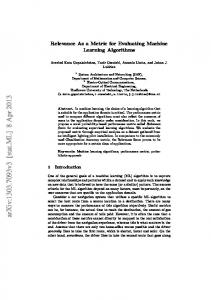
The basic building block of a neural network [17] such as a multilayer perceptron is a processing unit called a neuron (or simply node). The output of a neuron is a combination of the multiple inputs from other neurons. Each input is weighted by a weight factor. A neuron outputs or fires if the sum of the inputs exceeds a threshold function of the neuron. The output from a multiplayer perceptron is purely predictive. As there is no descriptive component, the resulting classification can be hard to understand (black box). The architecture of the multilayer perceptron consists of a single input layer of neurons, one or multiple hidden layers and a single output layer of neurons (see Figure 1). In order to learn the perceptron must adjust it weights. The learning algorithm compares the actual output to the desired output to determine the new weights repetitively for all training instances. The network trains with the standard backpropagation algorithm, which is a two-step procedure. The activity from the input pattern flows forward through the network, and the error signal flows backward to adjust the weights. The generalized delta rule adjusts the weights leading out of the hidden layer neurons and the weights leading into the output layer neurons. Using the generalized delta rule to adjust the weights leading to the hidden units is backpropagating the erroradjustment. Output Pattern
F O R W A R D
B A C K W A R D
A C T I V I T Y
E R R O R
Input Pattern
Figure 1: Backpropagation network
Our multiplayer perceptron uses sigmoid threshold functions. The number of input nodes is equal to the number of attributes and the number of output nodes is equal to the number of classes. There is only one hidden layer, which has as many nodes as the sum of the number of attributes and the number of classes divided by two. As we use different feature selection techniques that produce
March 2006
page 5 of 14
different feature subsets the number of input and hidden nodes differs depending on the number of features used. By default the algorithm we use performs normalisation of all attributes including the class attribute (all values are between -1 and +1 after the normalisation). The learning rate (weight change according to network error) was set to 0.3, the momentum (proportion of weight change from the last training step used in the next step) to 0.2 and we ran the training for 500 epochs (an epoch is the number of times training data is shown to the network).
is in fact a faster, more memory efficient solution to the QP problem vi. A more in depth treatment of the QP problem and the SMO solution are found in [23]. Implementing an SVM classifier requires the configuration of a number of parameters. Parameters we are most interested in are the complexity parameter C, the polynomial exponent p, for each of which we use the value of 1. The input space is also normalised before training.
G. Sequential Minimal Optimisation (SMO)
Boosting is a process used to increase the performance of weak learning algorithms. It can also be used on strong algorithms, but improvements are less dramatic. Boosting works by combining the classifiers produced by the learning algorithm over a number of distributions of the training data. We use an implementation of the AdaBoost algorithm developed in [18].
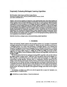
The SMO algorithm was developed as a faster, more scalable Support Vector Machine (SVM) [22]. These improvements are related to increasing the speed of training and as such classification is performed as with standard SVM. The basic process behind SVMs for classification is to map certain training data (xi,yi),i=1,…,l where each instance is characterized by a set of feature values xi∈Rn and a class label y∈{1,-1}l, into a higher-dimensional feature space Φ(x) for separation by a hyperplane. Support Vector Machines are binary classifiers, meaning only two types of data can be separated by one classification model. Multiple classifiers are created for multi-class scenarios. Figure 2 illustrates a linear SVM hyperplane separating two classes. Optimal Hyperplane
Margin of separation
Feature space
Figure 2: Optimal hyperplane and margin of separation
The linear algorithm can be evaluated in the feature space using the dot product Φ(x).Φ(y), although this is highly computational. Positive definite kernel functions k(x,y) have been shown to correspond to feature space dot products and are therefore substituted in place of the dot product:
k ( x, y ) = (Φ ( x) ⋅ Φ ( y )) .
(8)
H. AdaBoost
V. EXPERIMENTAL APPROACH This section describes the data and features that form the basis of our study as well as the software and performance metrics used in the evaluation. A. Traffic Classes
In our study a class represents an individual application. Example instances of each class are provided to the ML algorithm at training time. For accurate classification, the class instances used for training must be truly representative of the class. A drawback of using public anonymised trace files is the lack of payload data, making verification of the true application impossible. We chose a number of prominent applications (see Table 1) and selected the flows based on the IANA defined well-known ports (10,000 instances per class) and/or large feature would not be recommended due to large build times (several hundred hours would not be unusual). There was no particular search method that stood out as being greatly superior. Best first searches provide a slightly better accuracy with slightly less reduction of the feature set compared with greedy searches.
5 et BD 4. sN tN tC ye os os a o o B aB aB Ad Ad
5 4. C
LP M
BD N
N N
BK N
e re BT N
O SM
Figure 6: Mean accuracy of machine learning algorithms
B. Learning Algorithms
The mean accuracy of each algorithm across all feature subsets and traces is shown in Figure 6. The algorithms that stand out according to overall accuracy are Bayes Net, C4.5 and AdaBosot C4.5, followed by NBTree, AdaBoost NBD and Nearest Neighbour. MLP and SMO did not
CAIA Technical Report 060410B
The change in overall accuracy for each algorithm according to feature subset evaluation method, compared with the accuracy obtained using the full feature space is shown in Figure 7. A surprising result is the poor gains for NBK using the CFS selected subsets, as previous work [6] has shown this
March 2006
page 9 of 14
Accuracy
0.8 0.7
Mean Rate
0.9
Recall
0.6
15
Con
Wrapper 0.5
10
CFS
et N es ay B
5 4. C
LP M
BD N
N N
BK N
e Tr B N
e
O M S
0
5
5 D 4. B N C st st oo oo B B da da A A
BD N
N N
BK N
e re BT N
O M S
Figure 7: Average change in overall accuracy by subset selection method compared against using full feature set
The algorithms most sensitive to feature space reduction are MLP and SMO, which contributes to the low average accuracy seen in Figure 6. The decision trees showed comparatively small changes with feature selection. This is expected as tree-based algorithms essentially perform feature reduction as part of the learning process (the tree does not include irrelevant features). Bayes Net also shows relatively small changes in accuracy with feature selection. The Naive Bayes algorithms benefit most from using the wrapper technique. The mean accuracy in Figure 6 does not necessarily indicate the maximum performance of the algorithms, as some feature selection methods drastically reduced the average (the case for MLP and SMO). In addition, the accuracy distributions for all traces and search methods were consistent across the traces; it seems that no particular trace is harder or easier to classify then the others. Therefore, to decide which algorithm provides best accuracy we focus on the maximum achievable accuracies on the combined trace, and also examine class metrics Figure 8 plots the mean precision and recall rates and accuracy across the traffic classes for the combined trace and the feature subset that maximises the accuracy (determined by wrapper for Naive Bayes, otherwise the full feature set). Algorithms with very high overall accuracies also have high precision and recall values, with little difference between them. AdaBoost C4.5 (99.167%), C4.5 (98.643%) and NBTree (98.135%) achieved the highest overall accuracy. All other algorithms besides NBK, SMO and MLP achieved accuracies above 95%.
CAIA Technical Report 060410B
1.0
LP M
0.8
5 4. C
0.6
et N
0.4
es ay B
0.2
-20 5 D 4. B C N st st oo oo B B da da A A
To examine if particular traffic classes are harder to classify than others we create boxplot of the recall for each class obtained from all algorithms and traces using the full feature set (see Figure 9). The bottom of a box represents the 1st quartile, the line within a box is the median and the top represents the 3rd quartile. Whiskers extend 1.5 times the inter-quartile range and circles denote outliers. Most classes have very high recall across the algorithms. DNS in particular has very few outliers and a relatively narrow distribution. Telnet and FTP-data appear to be the most difficult to classify, with FTP-data having several significant outliers. However, the median values for each class are quite high, and a high recall is achieved for each when using one of the better performing algorithms.
Recall
-10
-5
Figure 8: Average precision and recall of all traffic classes and accuracy for the combined trace with best feature set
-15
change in accuracy (%)
Precision
1
combination to achieve 95% accuracy (using quite different features however). Accuracies in this region were only achieved using Naïve Bayes with discretised input data. Using a wrapper subset with kernel density estimation does show a large improvement, though. This may suggest that for our data some features are not well represented by continuous distributions.
FTP Data
Telnet
SMTP
DNS
HTTP
half-life
Figure 9: Recall for each traffic class using all features
Besides accuracy and tolerance to feature set reduction we have also defined several additional criteria to assess the algorithms: Classifications per second: The number of classifications the algorithm performs when testing the combined trace with all features. Speed is important to perform near real-time classification on large numbers of simultaneous networks flows. Build Time: The time required to build a classification model using the training dataset. Building the classifier can be done offline but as building times may reach
March 2006
page 10 of 14
54,700
23.77
Moderate
AdaBoostC4.5
11,188
266.99
Moderate
Nearest Neighbour
8
NA
Low
NBTree
5,974
1266.12
Moderate
Bayes Net
9,767
13.14
Moderatehigh
NBD
27,049
10.86
Low
AdaBoost NBD
1,908
158.24
Low
NBK
22.6
2.97
Low
SMO
28,958
115.84
Very High
MLP
14,394
2030.59
High
100
C4.5
99
Complexity
98
Build Time (seconds)
97
Classifications per second
96
Algorithm
95
Table 4: Performance and setup complexity by algorithm
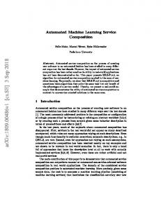
40,000, 200,000 or 400,000 samples of each class. The original combined dataset is also included for comparison. For traffic classes with flows less than the sample size, all flows were included. It should be noted that telnet, FTP-data, half-life and SMTP have a maximum of 1,727, 18,838, 107,227 and 241,251 flows respectively. This introduces some bias against these classes (as the algorithms optimise towards overall accuracy), but our goal here is to show the overall trend. The datasets were evaluated using 10-fold cross validation. Figure 10 shows an increase in accuracy with increasing sample size. The transition between 4,000 and 40,000 samples provides the largest increase in accuracy. The changes in accuracy are more or less proportionate between the three algorithms. Overall one might expect gains in accuracy to diminish as sample size increases. Gains above 200,000 samples per class came at a significant processing cost, as training times increased significantly with the larger sample size. Average Accuracy (%)
several days for certain classifiers, shorter build times may be more convenient. Setup Complexity: The effort required in configuring an algorithm and the possible level of ‘fine tuning’ required. Algorithms with many parameters must be tailored to specific datasets to achieve best performance, which can be a cumbersome process and can lead to over fitting. Performance metrics were measured using a 3.4 GHz Pentium 4 workstation with 4GB of RAM.
Bayes Net
Naive Bayes D
94
C4.5
4,000
200,000
400,000
Sample Size
D. Accuracy Depending on Flow Timeout
98 96 94 92
To investigate the influence of the size of the training dataset on the accuracy several new datasets were created using the stratified sampling method previously described. We use only C4.5, BayesNet and NBD, as they showed the best accuracy and also are considerably faster than slow algorithms such as MLP or NN. Feature selection was not performed for these datasets. The per-trace datasets contained up to 10,000, 50,000, or 100,000 flow samples of each traffic class. These datasets were then combined, creating datasets with up to
100
The original combined dataset was re-created with two new flow timeouts, 60 seconds and 1800 seconds, to compare the influence of flow timeout on classification performance. Short timeouts increase the number of UDP flows whereas long timeouts decrease the number of UDP flows. Although we use TCP semantics to detect flow termination still a number of TCP flows are terminated by timeouts. Short timeouts result in the chopping of some long-term TCP flows with large idle times. Figure 11 plots the overall accuracy depending on the timeout value.
C4.5
BayesNet
Naive Bayes D
90
C. Accuracy Depending on the Training Data Size
40,000
Figure 10: Overall accuracy by training data size
Accuracy (%)
Examining classifications per second, C4.5 has a considerable advantage, and is markedly faster than the closest algorithms, NBD, SMO and MLP. Nearest Neighbour is by far the slowest algorithm (a result of being a lazy learner). NBK is also very slow compared to the other algorithms. NBK provides the fastest build time of the algorithms, followed by Bayes Net and C4.5. NBTree and MLP have the longest training times. The increased accuracy of AdaBoost comes at a cost of speed, with AdaBoost C4.5 and AdaBoost NBD performing 7-17 times slower than the non-boosted versions.
60
600
1800
Timeout (s)
CAIA Technical Report 060410B
March 2006
page 11 of 14
Wrapper
All
80
Accuracy (%)
CON
70
1.00
60
0.98 0.96 0.94
5 4. C
s ye Ba
et N
BD N
Figure 13: Accuracy by subset selection method p2p traffic
0.92
Recall
CFS
90
100
Figure 11: Overall accuracy depending on flow timeout
The overall accuracy for each of the algorithms increases slightly with increasing flow timeout length. Figure 12 examines the recall for the individual traffic classes against flow timeout length for the C4.5 algorithm. These trends are similar for Bayes Net and NBD.
0.90
ftpdata telnet
SMTP DNS
HTTP half-life
60
600
1800
Timeout (s)
Figure 12: Recall depending on flow timeout per traffic class, C4.5 algorithm
The UDP flows (half-life and DNS) do not benefit from an increased flow timeout but the accuracy decrease is negligible. SMTP, FTP and HTTP applications benefit slightly moving from 60s to 600s, with little difference at 1800s. It is possible that these classes stay open-and-idle more than other classes, and thus benefit from having statistics from the entire flow. Against this trend, telnet sees a significant reduction in recall, probably a result of the significantly reduced number of flow instances (the 60s timeout has twice the number of training flows as for 1800s). An obvious drawback of using long flow timeouts is that there is a longer wait before a flow can be classified. Overall, the results suggest that in most cases accuracy is essentially unaffected by using short timeouts (e.g. 60 seconds). E. Accuracy for Peer-to-peer Traffic Classes
To determine whether our method of flow classification also extends to other traffic classes, we evaluate a dataset containing traffic of peer-to-peer file sharing applications. This dataset contains 1,000 flows of DNS, HTTP, eDonkey, BitTorrent and Kazaa. These flows are sampled from a trace hand-classified by using application protocol signatures. CFS, Consistency and wrapper subset evaluation were run for C4.5, Bayes Net and NBD algorithms. Figure 13 shows the accuracy depending on the feature selection technique and the ML algorithm.
CAIA Technical Report 060410B
Encouragingly the features selected by the three subset evaluation methods show a similar trend to those selected for the original classes. CFS was again biased towards packet length statistics, while Consistency preferred interarrival times. The ranking of subset evaluators is the same, with the wrapper method once more providing the highest accuracy. The ranking of the algorithms has changed: Bayes Net slightly outperformed C4.5. The maximum accuracies obtained for each algorithm are 98.98% for Bayes Net, 97.88% for C4.5 and 97.28% for NBD. VII. CONCLUSIONS AND FUTURE WORK In this paper we have evaluated the ability of different machine learning algorithms to identify network applications based on statistical payload-independent flow features. We show that there is great potential in using this method. With 22 features we are able to achieve classification accuracies of over 99% with two algorithms, and accuracies above 97% with several others. We also have evaluated three different feature selection techniques. We found that the wrapper method provides the best accuracy, but is slow to execute. It is able to improve accuracy over using the whole feature set, while still reducing the features space significantly. The filter methods are much faster but provide significantly less accuracy than using all features. CFS is generally faster and more accurate than the Consistency metric. Analysis of the selected features shows that packet length statistics and protocol are stronger class-discriminating features. The majority of algorithms perform very well with our datasets, obtaining high accuracies. Particularly strong algorithms are C4.5 (99.4%) and Bayes Net (99.3.2%), while NBTree (98.3%), NBD (98.3%) and Nearest Neighbour (97.7%) were also notable. The AdaBoost algorithm does provide some increases in accuracy (12%), but significantly slows down training and classification. Additional experiments show a short flow timeout of 60 seconds to be suitable, while increasing the training sample size shows significant improvement in accuracy. Tests on a dataset containing several popular peer-to-peer
March 2006
page 12 of 14
file sharing applications demonstrated that our technique could be expanded to other traffic classes. The results obtained are very promising, but there are a number of avenues to be further explored. We plan to investigate a wider range of flow features, including features based on multiple flows. We will also investigate classification accuracies achievable if only one direction of a flow can be observed. Additional classes, such as different online gaming applications, also need to be investigated. Tuning the parameters of the learning algorithms, especially for MLP and SMO, and evaluating the memory usage is also left for further studies. ACKNOWLEDGMENTS This paper has been made possible in part by a grant from the Cisco University Research Program Fund at Community Foundation Silicon Valley. REFERENCES [1] Thomas Karagiannis, Andre Broido, Nevil Brownlee, kc claffy, “Is P2P dying or just hiding?” In Proceedings of Globecom 2004, November/December 2004. [2] Tom M. Mitchell, “Machine Learning“, McGraw-Hill Education (ISE Editions), December 1997. [3] S. Zander, T.T.T. Nguyen, G. Armitage, “ Automated Traffic Classification and Application Identification using Machine Learning“, IEEE 30th Conference on Local Computer Networks (LCN 2005), Sydney, Australia, 15-17 November 2005. [4] M. Roughan, S. Sen, O. Spatscheck, N. Duffield, “Class-ofService Mapping for QoS: A statistical signature-based approach to IP traffic classification“, ACM SIGCOMM Internet Measurement Workshop, Sicily, Italy, 2004. [5] A. McGregor, M. Hall, P. Lorier, J. Brunskill, “Flow Clustering Using Machine Learning Techniques“, Passive & Active Measurement Workshop 2004 (PAM 2004), France, April 19-20, 2004. [6] A. W. Moore and D. Zuev, “Internet Traffic Classification Using Bayesian Analysis Techniques”, ACM SIGMETRICS, Banff, Canada, June 2005. [7] T. Karagiannis, K. Papagiannaki, and M. Faloutsos, “BLINC: Multilevel Traffic Classification in the Dark”, ACM Sigcomm, Philadelphia, PA, August 2005. [8] T. Dunnigan, G. Ostrouchov, “Flow Characterization for Intrusion Detection“, Technical Report, Oak Ridge National Laboratory, November 2000.
[11] M. Hall, “Correlation-based Feature Selection for Machine Learning“, PhD diss. Department of Computer Science, Waikato University, Hamilton, NZ, 1998. [12] WEKA 3.4.4, http://www.cs.waikato.ac.nz/ml/weka/ (March 2006). [13] R. Kohavi and J. R. Quinlan, Will Klosgen and Jan M. Zytkow, editors, “Decision-tree discovery”, In Handbook of Data Mining and Knowledge Discovery, chapter 16.1.3, pages 267-276, Oxford University Press, 2002. [14] G. H. John, P. Langley, “Estimating Continuous Distributions in Bayesian Classifiers”, 11th Conference on Uncertainty in Artificial Intelligence, pp. 338-345, Morgan Kaufman, San Mateo, 1995. [15] D. Aha, D. Kibler, “Instance-based learning algorithms”, In Machine Learning, vol. 6, pp. 37-66, 1991. [16] Ron Kohavi, “Scaling Up the Accuracy of Naive-Bayes Classifiers: a Decision-Tree Hybrid”, 2nd International Conference on Knowledge Discovery and Data Mining (KDD), 1996. [17] C. M. Bishop, “Neural Networks for Pattern Recognition”, Oxford University Press, 1995. [18] Y. Freund, R. E. Shapire, “Experiments with a new boosting algorithm”, International Conference of Machine Learning, pp. 148-156, San Francisco, 1996. [19] NetMate, http://sourceforge.net/projects/netmate-meter/ (March 2006). [20] NLANR traces: http://pma.nlanr.net/Special/ (March 2006). [21] R. Bouckaert, “Bayesian Network Classifiers in Weka”, Technical Report, Department of Computer Science, Waikato University, Hamilton, NZ 2005. [22] J. C. Platt, “Sequential Minimal Optimization: A Fast Algorithm for Training Support Vector Machines”, Technical Report MSRTR-98-14, Microsoft Research, April 1998. [23] G. Cawley, “Efficient Sequential Minimal Optimisation of Support Vector Classifiers”, Technical Report, School of Information Systems, University of East Angila, Norwich, Norfolk, UK, 2001 [24] D. E. Goldberg, "Genetic Algorithms in Search, Optimization, and Machine Learning", Addison-Wesley, 1989. [25] N. Brownlee, “NeTraMet & NeMaC Reference Manual”, University of Auckland, http://www.auckland.ac.nz/ net/Accounting/ntmref.pdf, June 1999.
[9] M. A. Hall, G. Holmes, “Benchmarking attribute selection techniques for discrete class data mining“, IEEE Transactions on Knowledge & Data Engineering, Vol 15, No 6, pp 1437-1447, 2003. [10] M. Dash, H. Liu, “Consistency-based search in feature selection”, Artificial Intelligence, 151:155-176, 2003.
CAIA Technical Report 060410B
March 2006
page 13 of 14
APPENDIX The complete list of flow features and their abbreviations:
Mean forward inter-arrival time
meanfiat
Maximum forward inter-arrival time
maxfiat
Standard deviation of forward inter-arrival times
stdfiat
Feature Description
Abbreviation
Minimum backward inter-arrival time
minbiat
Minimum forward packet length
minfpktl
Mean backward inter-arrival time
meanbiat
Mean forward packet length
meanfpktl
Maximum backward inter-arrival time
maxbiat
Maximum forward packet length
maxfpktl
Standard deviation of backward inter-arrival times
stdbiat
Standard deviation of forward packet length
stdfpktl
Protocol
protocol
Minimum backward packet length
minbpktl
Duration of the flow
duration
Mean backward packet length
meanbpktl
Number of packets in forward direction
fpackets
Maximum backward packet length
maxbpktl
Number of bytes in forward direction
fbytes
Standard deviation of backward packet length
stdbpktl
Number of packets in backward direction
bpackets
Minimum forward inter-arrival time
minfiat
Number of bytes in backward direction
bbytes
CAIA Technical Report 060410B
March 2006
page 14 of 14