Journal of Information Security, 2015, 6, 250-264 Published Online July 2015 in SciRes. http://www.scirp.org/journal/jis http://dx.doi.org/10.4236/jis.2015.63025
Evaluation of Modified Vector Space Representation Using ADFA-LD and ADFA-WD Datasets Bhavesh Borisaniya, Dhiren Patel Computer Engineering Department, NIT Surat, India Email:
[email protected],
[email protected] Received 10 June 2015; accepted 25 July 2015; published 28 July 2015 Copyright © 2015 by authors and Scientific Research Publishing Inc. This work is licensed under the Creative Commons Attribution International License (CC BY). http://creativecommons.org/licenses/by/4.0/
Abstract Predicting anomalous behaviour of a running process using system call trace is a common practice among security community and it is still an active research area. It is a typical pattern recognition problem and can be dealt with machine learning algorithms. Standard system call datasets were employed to train these algorithms. However, advancements in operating systems made these datasets outdated and un-relevant. Australian Defence Force Academy Linux Dataset (ADFA-LD) and Australian Defence Force Academy Windows Dataset (ADFA-WD) are new generation system calls datasets that contain labelled system call traces for modern exploits and attacks on various applications. In this paper, we evaluate performance of Modified Vector Space Representation technique on ADFA-LD and ADFA-WD datasets using various classification algorithms. Our experimental results show that our method performs well and it helps accurately distinguishing process behaviour through system calls.
Keywords System Call Trace, Vector Space Model, Modified Vector Space Representation, ADFA-LD, ADFA-WD
1. Introduction System call is a request for a service that program makes to the kernel. Sequence of the system calls can describe the behaviour of the process. System call traces are used in Host based Intrusion Detection System (HIDS) to distinguish normal and malicious processes. There are a number of data representation techniques found in literature (e.g, n-gram model and lookahead pairs [1] [2], sequencegram [3], pairgram [4], etc.) used to extract the features from the system call trace for process behaviour classification.
How to cite this paper: Borisaniya, B. and Patel, D. (2015) Evaluation of Modified Vector Space Representation Using ADFA-LD and ADFA-WD Datasets. Journal of Information Security, 6, 250-264. http://dx.doi.org/10.4236/jis.2015.63025
B. Borisaniya, D. Patel
By considering collected system call traces as set of document and system calls as words, we can apply classical data representation and classification techniques used in the area of natural language processing (NLP) and information retrieval (IR). Document representation techniques such as Boolean model and vector space model were reported in literature for extracting features from system call traces. X. Wang et al. [5] used n-gram with Boolean model for feature extraction and Support Vector Machine (SVM) with Gaussian Radial Basis Function (GRBF) kernel function for classification. K. Rieck et al. [6] used vector space model and considered frequency of system call in a trace as a weight of system call. They utilized polynomial kernel function for classifying the vectors storing weight of each system call. Y. Liao and V. R. Vermuri [7] have used vector space model for system call trace representation and applied k-nearest neighbour (kNN) classifier, where nearness was calculated using cosine similarity. However, these approaches are not considering system call sequence information, which would help in better describing the system call behaviour. Researchers were utilizing the well-known system call trace datasets like University of New Maxico (UNM) intrusion detection dataset [8], and DARPA intrusion detection dataset [9] to train the machine learning algorithms for process behaviour prediction. However, these datasets were compiled decades ago and are not very relevant for modern operating systems [10]. Recently (in 2013), new system call trace datasets released by G. Creech et al. known as ADFA datasets [10] [11]. ADFA datasets are considered as new benchmark for evaluating system call based intrusion detection systems. It has a wide collection of system call traces representing modern vulnerability exploits and attacks. G. Creech et al. [12] have proposed semantic model for anomaly detection using short sequences of ADFALD Dataset. They have prepared the dictionary of word and phrase from the dataset and evaluated it with the Hidden Markov Model (HMM), Extreme Learning Machine (ELM) and one-class SVM algorithms. They achieve accuracy of 90% for ELM and 80% for SVM with 15% false positive rate (FPR) [12] [13]. For ADFAWD evaluation also, G. Creech et al. [11] have used HMM, ELM and SVM. They noted 100% accuracy with 25.1% FPR for HMM, 91.7% accuracy with 0.23% FP rate with ELM and 99.58% accuracy with 1.78% FP rate for SVM. However, learning a dictionary of all possible short sequences is a time consuming task [14] [15]. Miao Xie et al. [15] have applied k-nearest neighbour (kNN) and k-means clustering (kMC) algorithms on ADFA-LD dataset. They considered frequency based model for data representation and used principal component analysis (PCA) to reduce the dimension of feature vector. With combination of kNN and kMC they achieve accuracy of 60% with 20% of FPR. In another attempt Miao Xie et al. [13] have applied one-class SVM with short sequence based technique on ADFA-LD. With one-class SVM, they achieved maximum accuracy of 70% with around 20% of FPR. We modified the X. Wang et al. [5] approach given for Boolean model and proposed Modified Vector Space Representation in [16] to represent process system call trace in terms of feature vector. It is system call frequency based approach and utilizes the Vector Space Model with n-gram. In [16], we have evaluated the proposed method on system call trace datasets used in [17]. In this paper, we apply modified vector space representation approach on ADFA-LD and ADFA-WD dataset and discuss results obtained with the help of different classification techniques chosen for evaluation. Rest of the paper is organized as follows: Section 2 describes classic data representation techniques in context of system call trace with their limitations. Section 3 discusses modified vector space representation. Section 4 details the datasets, algorithms selected, chosen evaluation metrics and experiments methodology used for evaluation. Section 5 discusses the performance results followed by conclusion and references at the end.
2. System Call Trace Representation In order to classify the process behaviour using system call trace, one needs to extract the features from it. Data representation techniques can be used to convert the system call trace into feature vector. Common data representation techniques used for system call representation are as follows:
2.1. Trivial Representation The basic representation of system call trace is to consider it as a string (sequence) of system calls. Let us consider an operating system with total m number of unique system calls, then set of system calls can be represented by U = {s1 , s2 , s3 , , sm } . Let Fi be finite sequence of system calls and U * represents the set of all * possible finite sequences of system calls then Fi ∈ U and Fi represents the length of the sequence. N is the
251
B. Borisaniya, D. Patel
total number of applications (normal and malware) used in training and testing for analysis. D is the dataset containing system call traces of selected applications and formally defined= as D
{ S ,L i
i
1 ≤ i ≤ N , Si ∈ U * ,
Li ∈ {normal, malware}} , where Si is a system call trace of i th application and Li is its label (i.e. normal or
(
)
malware). The memory complexity for such representation is O N × ∑ i =1 Si . Here N
∑ i =1 Si N
represents the
total length of sequences. If length of system call sequences is large, this could be a big number.
2.2. Boolean Model Simple representation technique can be found in the area of information retrieval is Boolean Model [18]. It is an exact match model, which can represent a system call trace as a vector having all possible system call number as its index. The value of index is 1 if system call is present in given trace and 0 otherwise. Consider total number of system calls in an operating system is m. A system call trace Si can be represented using boolean model as a feature vector A = b1 , b2 , b3 , , bm , where, m = U and b j ∈ {0,1} ,1 ≤ j ≤ m . The memory complexity of Boolean model is O ( N × U ) . This model considers every system call equally important and only marks its presence or absence. It does not assign any weight to the system call that appears multiple times in a system call trace.
2.3. Vector Space Model Vector Space Model is another common and powerful technique used in information retrieval field to represent document as set of words [18]. It is also known as “bag of words” technique as it assigns weight to each word in the given document in order to determine how much the document is relevant to specific words. Here the weight is assigned to a word as number of times the word appear in the document. In the context of system call representation, system call trace is considered as document and each system call as one word. Then we can apply vector space model to represent given system call trace as a feature vector. To represent the system call traces using vector space model (bag of words) representation, let us consider a feature set B, as a set of vectors corresponds to applications’ system call traces. System call trace for an application i with this model can be represented as, vector Bi = n1 , n2 , n3 , , nm , where m = U and n j (1 ≤ j ≤ m ) represents the number of times the system call s j appears in the system call trace sequence Si . The memory complexity of vector space model representation is similar to Boolean model i.e. O ( N × U ) . Here, U is number of system calls. For example, Linux 3.2 has 349 system calls, then U = 349. Note that, N number of system calls U is smaller than total length of sequences ∑ i =1 Si if system call sequence Si is large.
3. Modified Vector Space Representation Vector space model cannot preserve the relative order of system calls. e.g. Feature vector for system call traces S1 : open, read , close, exit and S2 : open, exit , close, read are similar. Relative order of system calls is more important in case of modelling process behaviour. Loss of system call sequence information can leave a system vulnerable to mimicry attacks [19] [20], where a malware writer interleaves malware system call trace patterns with benign system call trace. Thus, we consider the multiple consecutive system calls as one term. Number of system calls in a term is defined by term-size. For term-size l and total number of unique system calls m, n-gram model provide total ml number of possible unique terms in a feature vector. In order to represent the system call traces using this approach, let us consider U l be the set of all possible l unique terms of length (term-size) l. Here, U l = {t1 , t2 , t3 , , tr } , where= r U = ml and tk (1 ≤ k ≤ r ) repreth sents the k term of length l derived through n-gram model from U. The feature set C contains the occurrence of each term in given system call trace. For instance, Ci = n1 , n2 , n3 , , nr , where nk (1 ≤ k ≤ r ) represents the number of times the term tk appears in the system call trace Si . The memory requirement for n-gram with l vector space model approach for term length of l is O N × U . l Representation created using n-gram model is more costly than normal vector space model as U < U . In addition to that, all features (terms) are not present in the system call traces, which means they are having zero weight in feature vector. We can reduce the dimension of feature vector by considering only those unique terms
(
252
)
B. Borisaniya, D. Patel
which are present in the data. If we consider only those unique terms that appear in training data, the memory requirement would be less compared to considering all possible unique terms generated from U. This can be represented by set of all unique l l terms of length l occurring in training data. The set can be defined as U train ⊂ U l , where, U train is a set of only l those terms, appearing in training dataset. Here the number of terms in feature set U train would be less coml l ≤ U . Considering, N train as number of pared to all possible terms of length l generated from U i.e. U train l . system call traces in training dataset, memory complexity of this representation would be O N train × U train However, this representation does not cover system call sequences, which were not explored during training and may appear in testing. The feature vector built by considering only those terms that appeared in training data is much compact than other system call representations. However, it requires prior knowledge of unique terms in system call traces, which is not always possible. We can easily find the unique terms from the training data. However, during training, we might not have explored all possible usages of application. It is quite possible that, terms that were not present in the training data may appear in testing data. Modified Vector Space Representation [16] extends the previous representation (which considers unique terms from training data only) by incorporating mechanism to handle any unforeseen terms during testing. We deliberately add a system call number (we refer it as unknown (unk)) in list, whose value is higher than any system call number present in system call list for OS. We form terms of length l comprising this unknown system call number including one term having all unknown system call number. Let E be the set of unknown terms comprising unk system call number. unk is a number deliberately added in the list of system call numbers to map terms, which are not seen during training but found in testing. Hence, the new feature set can be l l l is set comprises of all unique terms of length l appearing in traindefined as U new = U train E , where U new l ing data U train and set of terms having unk system call number E. Considering, N train as number of system
(
(
)
)
l call trace sequences in training, memory complexity of this representation would be O N train × U new , where
U = U l new
l train
+ E . Here, number of terms comprising of unk system call E will be very small.
4. Evaluation In this section we provide details of datasets, classification algorithms selected, evaluation metrics and experiments methodology used for evaluation.
4.1. Datasets We have evaluated modified vector space representation with two datasets namely ADFA-LD (Linux Dataset) and ADFA-WD (Windows Dataset) constructed by G. Creech et al. [10]-[12]. Table 1 describes the number of traces collected from [21] for each category for ADFA-LD and ADFA-WD dataset. For ADFA-LD system call traces for specific process were generated using auditd [22] Unix program, an auditing utility for collecting security relevant events. These traces were then filtered for undersize and oversize limit, which is 300 Bytes to 6 kB for training data and 300 Bytes to 10 kB for validation data [11] [12]. ADFA-LD dataset was collected under Ubuntu 11.04 fully patched operating system with kernel 2.6.38. The operating system was running different services like webserver, database server, SSH server, FTP server etc. ADFA-LD also incorporates system call traces of different types of attacks. Table 2 describes details of each attack class in ADFA-LD dataset [11] [12]. Table 1. Number of system call traces in different category of ADFA-LD and ADFA-WD dataset. ADFA-LD
ADFA-WD
Dataset Training data Validation data Attack data Total
Traces
System Calls
Traces
System Calls
833
3,08,077
355
1,35,04,419
4,372
21,22,085
1,827
11,79,18,735
746
3,17,388
5,542
7,42,02,804
5,951
27,47,550
7,724
20,56,25,958
253
B. Borisaniya, D. Patel
Table 2. Attack vectors used to generate ADFA-LD attack dataset. Attack
Payload/Effect
Vector
Trace Count
Hydra-FTP
Password bruteforce
FTP by Hydra
162
Hydra-SSH
Password bruteforce
SSH by Hydra
176
Adduser
Add new superuser
Client side poisoned executable
Java-Meterpreter
Java based Meterpreter
TikiWiki vulnerability exploit
Meterpreter
Linux Meterpreter Payload
Client side poisoned executable
Webshell
C100 Webshell
PHP remote file inclusion vulnerability
91 124 75 118
ADFA-WD (Windows Dataset) represents the high-quality collection of DLL access requests and system calls for a variety of hacking attacks [11]. Dataset was collected in Windows XP SP2 host with the help of Procmon [23] program. Default firewall was enabled and Norton AV 2013 was installed to filter only sophisticated attacks and ignore the low level attacks. The OS environment enabled file sharing and configured network printer. It was running applications like, webserver, database server, FTP server, streaming media server, PDF reader, etc. Total 12 known vulnerabilities for installed applications were exploited with the help of Metasploit framework and other custom methods. Table 3 describes the details of each attack class in ADFA-WD dataset [11].
4.2. Algorithms Selected for Experiments We selected Weka workbench [24] [25] for evaluation of modified vector space representation on ADFA-LD and ADFA-WD datasets. Weka hosts number of machine learning algorithms which can be easily applied on our prepared datasets of varying term-size. We selected nine well-known classification algorithms from six different categories given in Weka. The list of selected algorithms, selected options for individual algorithm and their respective category in Weka are shown in Table 4.
4.3. Experiments Methodology Datasets were collected from [21] and then converted into modified vector space representation for various term-size. For these experiments we selected the term-size 1, 2, 3 and 5. For each dataset (i.e. ADFA-LD and ADFA-WD) we ran experiments for binary class as well as for multiclass label classification. For binary class we considered one of two labels for each trace - normal and attack. For multiclass classification, number of classes and class labels are different for both datasets. In ADFA-LD we have total 7 class labels viz. normal, adduser, hydra-ftp, hydra-ssh, java-meterpreter, meterpreter and webshell. While in ADFA-WD we have total 13 class labels viz. normal and V1 to V12. We ran each chosen algorithms with selected options on converted data in Weka through 10-fold cross-validation method. Table 5 describes the number of features extracted from ADFA-LD and ADFA-WD dataset for varying term-size using modified vector space representation.
4.4. Evaluation Metrics We have used the following common evaluation metrics that are widely used in information retrieval area [18]: True Positive (TP): Number of attack traces detected as attack traces. False Positive (FP): Number of attack traces detected as normal traces. True Negative (TN): Number of normal traces detected as normal traces. False Negative (FN): Number of normal traces detected as attack traces. Figure 1 shows the confusion matrix, which can be used to derive other measures. Precision: It is the ratio of how many attack traces predicted as attack traces out of total number of traces predicted as attack traces. TP Precision = TP + FP
254
B. Borisaniya, D. Patel
Table 3. Vulnerabilities considered to generate ADFA-WD attack dataset. ID
Vulnerability
Program
Exploit Mechanism
V1
CVE: 2006-2961
CesarFTP 0.99g
Reverse Ordinal Payload Injection
Trace Count 454
V2
EDB-ID: 18367
XAMPP Lite v1.7.3
Upload and execute malicious payload using Xampp_webdav
470
V3
CVE: 2004-1561
Icecast v2.0
Metasploit exploit
382
V4
CVE: 2009-3843
Tomcat v6.0.20
Metasploit exploit
418
V5
CVE: 2008-4250
OS SMB
Metasploit exploit
355
V6
CVE: 2010-2729
OS Print Spool
Metasploit exploit
454
V7
CVE: 2011-4453
PMWiki v2.2.30
Metasploit exploit
430
V8
CVE: 2012-0003
Wireless Karma
DNS Spoofing using Pineapple Router
487
V9
CVE: 2010-2883
Adobe Reader 9.3.0
Reverse Shell spawn through malicious PDF
440
V10
-----
Backdoor executable
Reverse Inline Shell spawned
536
V11
CVE: 2010-0806
IE v6.0.2900.2180
Metasploit exploit
495
V12
-----
Infectious Media
Blind Shell spawned
621
Table 4. List of selected algorithms with their options. Category
Algorithm
Option(s) Selected
Bayes
Naïve Bayes
---
SMO (Sequential Minimal Optimization)
Polynomial Kernel
LibSVM (Support Vector Machine)
Radial Basis Function (RBF) Kernel, gamma = 0.5, loss = 0.001
Lazy
IBk (k-nearest neighbors)
k = 1, 2, 3
Meta
Classification via ClusteringSimple K Means (k Means)
k = 2 (7 and 13 for multiclass classification on ADFA-LD and ADFA-WD dataset respectively)
ZeroR
---
OneR
minBucketSize(B) = 5, 6, 10
JRip (RIPPER)
Folds = 3
J48 (C4.5)
confidenceFactor = 0.25, minNumObj = 2
Function
Rules
Trees
Table 5. Number of features extracted from ADFA-LD and ADFA-WD dataset for term-size 1, 2, 3 and 5. term-size Dataset 1
2
3
5
ADFA-LD
175
3,792
24,818
1,63,263
ADFA-WD
1,309
4,801
13,472
42,426
Figure 1. Confusion matrix.
255
B. Borisaniya, D. Patel
Recall: Recall also known as the True Positive Rate (TPR). It is the ratio of how many attack traces predicted as attack traces out of total number of actual attack traces.
Recall =
TP TP + FN
Accuracy: Accuracy is the proportion of true results (number of attack traces and normal traces detected correctly) in the total number of samples.
Accuracy =
TP + TN TP + FP + TN + FN
FP Rate: False Positive Rate (FPR) is a measure of how many normal trace are labelled as attack trace by classifier.
FPRate =
FP FP + TN
F-Measure: It is a measure that combines precision and recall into a single measure. It is calculated as harmonic mean of precision and recall.
F-Measure =
2 1 1 + Precision Recall
Receiver Operating Characteristics (ROC) Curve: It is a graph of true positive rate against false positive rate. It represents the performance of binary classifier as its discrimination threshold is varied. Area Under the ROC Curve (AUC): It is the area covered by ROC curve. It is equivalent to the probability that a classifier will rank a randomly chosen positive instance higher than a randomly chosen negative one [26].
5. Results and Analysis Figure 2 shows the performance results in terms of accuracy and false positive rate of selected algorithms with varying term-size on both datasets. The results shown here are the weighted average of results derived for individual class labels. Detailed experiment (weighted average) results on ADFA-LD and ADFA-WD are given in Appendix (Tables A1-A4). From Figure 2, we can observe that using modified vector space representation all algorithms perform reasonably well. However, IBk and J48 performed best in all experiments. With IBk algorithm we can notice that as we increase the term-size, its performance starts degrading (i.e. accuracy decreases and FP Rate increases). These changes are clearly visible in case of ADFA-LD dataset. Similar performance results are achieved by J48 in all experiments. However, IBk have higher FP Rate compare to J48 for term-size 3 and 5 on ADFA-LD dataset. Comparing IBk and J48 with application perspective, J48 requires more time in building the decision tree model during training but it is faster during testing phase. On contrary, IBk does not have any difference between training and testing phase. It finds distance between test instance and all other training instances during testing phase. Due to this IBk seeks high amount of memory space to store all training instances during testing phase compare to J48, whereas storing J48 model is merely a tree to be stored. So, with J48 in testing phase classifying a test instance is as simple as traversing limited number of branches (based on feature values) of a decision tree from root to leaf. On ADFA-WD dataset, all algorithms perform well for binary class classification, but perform poorly for multiclass classification. Similar facts can be observed from Figure 3 and Figure 4. Figure 3 shows ROC curves of IBk (k = 1) and J48 with all term-size on ADFA-LD and ADFA-WD datasets for binary class classification. Figure 4 shows ROC curves of IBk (k = 1) and J48 with term-size 3 on ADFA-LD and ADFA-WD datasets for multiclass classification. From Figure 4(c), Figure 4(d) and Table A4 we can observe that IBk and J48 achieves high accuracy for normal class on ADFA-WD, but fails to distinguish among attack classes. The
256
B. Borisaniya, D. Patel
Figure 2. Performance results (FP rate and accuracy) of selected algorithms on ADFA-LD and ADFAWD dataset with binary class and multiclass classification for varying term-size. (a) FP rate—ADFA-LD (binary class); (b) Accuracy— ADFA-LD (binary class); (c) FP rate—ADFA-LD (multiclass); (d) Accuracy—ADFA-LD (multiclass); (e) FP rate— ADFA-WD (binary class); (f) Accuracy—ADFA-WD (binary class); (g) FP rate—ADFA-WD (multiclass); (h) Accuracy—ADFA-WD (multiclass).
257
B. Borisaniya, D. Patel
Figure 3. ROC curves of IBk (k = 1) and J48 on ADFA-LD and ADFA-WD with various term-size for binary class classification. (a) IBk (k = 1) on ADFA-LD; (b) J48 on ADFA-LD; (c) IBk (k = 1) on ADFA-WD; (d) J48 on ADFA-WD.
possible cause for this could be, similarity among system call traces of vulnerabilities exploits launched through metasploit.
6. Conclusion In this work, we have evaluated our proposed modified vector space representation using ADFA-LD and ADFA-WD system call trace datasets. We extracted features from both datasets using our proposed method for varying term-size. We also considered binary class and multiclass classification for evaluation on both datasets. Modified vector space representation (term-size 2, 3 and 5) performs as well as standard vector space model (term-size 1) if not better in terms of accuracy, FP rate and F-measure. There is no significant difference in results for varying term-size. However, higher term-size preserves more system call sequence information, which provides resistance against mimicry attacks. From the evaluation results, we conclude that IBk and J48 perform better on both datasets compare with other selected algorithms.
258
B. Borisaniya, D. Patel
Figure 4. ROC curves of IBk (k = 1) and J48 with term-size 3 on ADFA-LD and ADFA-WD for multiclass classification. (a) IBk (k = 1) on ADFA-LD; (b) J48 on ADFA-LD; (c) IBk (k = 1) on ADFA-WD; (d) J48 on ADFA-WD.
References [1]
Forrest, S., Hofmeyr, S.A., Somayaji, A. and Longstaff, T.A. (1996) Sense of Self for Unix Processes. Proceedings of the 1996 IEEE Symposium on Security and Privacy, Oakland, 6-8 May 1996, 120-128. http://dx.doi.org/10.1109/SECPRI.1996.502675
[2]
Hofmeyr, S.A., Forrest, S. and Somayaji, A. (1998) Intrusion Detection Using Sequences of System Calls. Journal of Computer Security, 6, 151-180. http://dl.acm.org/citation.cfm?id=1298081.1298084
[3]
Hubballi, N., Biswas, S. and Nandi, S. (2011) Sequencegram: n-Gram Modeling of System Calls for Program Based Anomaly Detection. 2011 Third International Conference on Communication Systems and Networks (COMSNETS 2011), Bangalore, 4-8 January 2011, 1-10. http://dx.doi.org/10.1109/COMSNETS.2011.5716416
[4]
Hubballi, N. (2012) Pairgram: Modeling Frequency Information of Lookahead Pairs for System Call Based Anomaly Detection. Fourth International Conference on Communication Systems and Networks (COMSNETS 2012), Bangalore, 3-7 January 2012, 1-10. http://dx.doi.org/10.1109/COMSNETS.2012.6151337
[5]
Wang, X., Yu, W., Champion, A., Fu, X. and Xuan, D. (2007) Detecting Worms via Mining Dynamic Program Execution. Proceedings of Third International Conference on Security and Privacy in Communications Networks and the Work-
259
B. Borisaniya, D. Patel
shops (SecureComm 2007), Nice, 17-21 September 2007, 412-421. http://dx.doi.org/10.1109/SECCOM.2007.4550362
[6]
Rieck, K., Holz, T., Willems, C., Düssel, P. and Laskov, P. (2008) Learning and Classification of Malware Behavior. Detection of Intrusions and Malware, and Vulnerability Assessment, LNCS, 5137, 108-125. http://dx.doi.org/10.1007/978-3-540-70542-0_6
[7]
Liao, Y. and Vemuri, V.R. (2002) Using Text Categorization Techniques for Intrusion Detection. USENIX Security Symposium, USENIX Association, Berkeley, 51-59. https://www.usenix.org/legacy/events/sec02/full_papers/liao/liao.pdf
[8]
Forrest, S. University of New Mexico (UNM) Intrusion Detection Dataset. http://www.cs.unm.edu/~immsec/systemcalls.htm
[9]
DARPA Intrusion Detection Dataset. http://www.ll.mit.edu/ideval/data/
[10] Creech, G. and Hu, J. (2013) Generation of a New IDS Test Dataset: Time to Retire the KDD Collection. Wireless Communications and Networking Conference (WCNC 2013), Shanghai, 7-10 April 2013, 4487-4492. http://dx.doi.org/10.1109/WCNC.2013.6555301 [11] Creech, G. (2014) Developing a High-Accuracy Cross Platform Host-Based Intrusion Detection System Capable of Reliably Detecting Zero-Day Attacks. Ph.D. Dissertation, University of New South Wales, Sydney. http://handle.unsw.edu.au/1959.4/53218 [12] Creech, G. and Hu, J. (2014) A Semantic Approach to Host-Based Intrusion Detection Systems Using Contiguous and Discontiguous System Call Patterns. IEEE Transactions on Computers, 63, 807-819. http://dx.doi.org/10.1109/TC.2013.13 [13] Xie, M., Hu, J. and Slay, J. (2014) Evaluating Host-Based Anomaly Detection Systems: Application of the One-Class SVM Algorithm to ADFA-LD. Proceedings of the 11th IEEE International Conference on Fuzzy Systems and Knowledge Discovery (FSKD 2014), Xiamen, 19-21 August 2014, 978-982. http://dx.doi.org/10.1109/fskd.2014.6980972 [14] Xie, M. and Hu J. (2013) Evaluating Host-Based Anomaly Detection Systems: A Preliminary Analysis of ADFA-LD. Proceedings of the 6th IEEE International Congress on Image and Signal Processing (CISP 2013), Hangzhou, 16-18 December 2013, 1711-1716. http://dx.doi.org/10.1109/CISP.2013.6743952 [15] Xie, M., Hu, J., Yu, X. and Chang, E. (2014) Evaluating Host-Based Anomaly Detection Systems: Application of the Frequency-Based Algorithms to ADFA-LD. Proceedings of 8th International Conference on Network and System Security (NSS 2014), Lecture Notes in Computer Science, 8792, 542-549. http://dx.doi.org/10.1007/978-3-319-11698-3_44 [16] Borisaniya, B., Patel, K. and Patel, D. (2014) Evaluation of Applicability of Modified Vector Space Representation for in-VM Malicious Activity Detection in Cloud. Proceedings of the 11th Annual IEEE India Conference (INDICON 2014), Pune, 11-13 December 2014, 1-6. http://dx.doi.org/10.1109/INDICON.2014.7030588 [17] Canali, D., Lanzi, A., Balzarotti, D., Kruegel, C., Christodorescu, M. and Kirda, E. (2012) A Quantitative Study of Accuracy in System Call-Based Malware Detection. Proceedings of the 2012 International Symposium on Software Testing and Analysis (ISSTA 2012), Minneapolis, 15-20 July 2012, 122-132. http://dx.doi.org/10.1145/2338965.2336768 [18] Manning, C., Raghavan, P. and Schütze, H. (2008) Introduction to Information Retrieval. Cambridge University Press, Cambridge. http://www-nlp.stanford.edu/IR-book http://dx.doi.org/10.1017/CBO9780511809071 [19] Wagner, D. and Dean, D. (2001) Intrusion Detection via Static Analysis. Proceedings of the 2001 IEEE Symposium on Security and Privacy, Oakland, 14-16 May 2001, 156-168. http://dx.doi.org/10.1109/secpri.2001.924296 [20] Wagner, D. and Soto, P. (2002) Mimicry Attacks on Host-Based Intrusion Detection Systems. Proceedings of the 9th ACM Conference on Computer and Communications Security (CCS 2002), Washington DC, 18-22 November 2002, 255-264. http://dx.doi.org/10.1145/586110.586145 [21] The ADFA Intrusion Detection Datasets. http://www.cybersecurity.unsw.adfa.edu.au/ADFA IDS Datasets/ [22] Auditd. http://linux.die.net/man/8/auditd [23] Process Monitor (Procmon). https://technet.microsoft.com/en-us/library/bb896645.aspx [24] Holmes, G., Donkin, A. and Witten, I.H. (1994) WEKA: A Machine Learning Workbench. Proceedings of the 1994 Second Australian and New Zealand Conference on Intelligent Information Systems, Brisbane, 29 November-2 December 1994, 357-361. http://www.cs.waikato.ac.nz/ihw/papers/94GH-AD-IHW-WEKA.pdf http://dx.doi.org/10.1109/ANZIIS.1994.396988 [25] Weka. http://www.cs.waikato.ac.nz/ml/weka/ [26] Fawcett, T. (2006) An Introduction to ROC Analysis. Pattern Recognition Letters, 27, 861-874. http://dx.doi.org/10.1016/j.patrec.2005.10.010
260
B. Borisaniya, D. Patel
Appendix: Experiment Results
In this section we provide detailed experiment results on ADFA-LD and ADFA-WD with binary class and multiclass class labels. Results shown here are weighted average results of individual class results. Table A1. Experiment results for various term-size on ADFA-LD dataset with binary class labels. Algorithm Naïve Bayes
SMO
LibSVM
IBk (k = 1)
IBk (k = 2)
IBk (k = 3)
kMeans (k = 2)
ZeroR
OneR (B = 5)
OneR (B = 6)
OneR (B = 10)
JRip
J48
term-size 1 2 3 5 1 2 3 5 1 2 3 5 1 2 3 5 1 2 3 5 1 2 3 5 1 2 3 5 1 2 3 5 1 2 3 5 1 2 3 5 1 2 3 5 1 2 3 5 1 2 3 5
FP Rate 0.083 0.088 0.102 0.251 0.765 0.258 0.226 0.305 0.844 0.845 0.847 0.847 0.124 0.136 0.155 0.126 0.188 0.223 0.388 0.564 0.144 0.193 0.387 0.574 0.858 0.865 0.863 0.865 0.875 0.875 0.875 0.875 0.759 0.733 0.656 0.647 0.773 0.73 0.657 0.637 0.778 0.719 0.656 0.635 0.168 0.18 0.205 0.274 0.154 0.176 0.219 0.266
Precision 0.902 0.914 0.926 0.917 0.863 0.943 0.946 0.934 0.885 0.884 0.884 0.884 0.96 0.957 0.926 0.912 0.96 0.956 0.916 0.894 0.959 0.95 0.904 0.885 0.749 0.75 0.745 0.776 0.765 0.765 0.765 0.765 0.833 0.846 0.884 0.881 0.846 0.846 0.886 0.884 0.886 0.848 0.884 0.885 0.957 0.955 0.953 0.939 0.959 0.958 0.95 0.941
261
Recall 0.699 0.818 0.882 0.91 0.883 0.945 0.948 0.938 0.879 0.879 0.878 0.878 0.96 0.956 0.906 0.844 0.961 0.957 0.922 0.905 0.959 0.95 0.909 0.899 0.722 0.771 0.863 0.865 0.875 0.875 0.875 0.875 0.871 0.877 0.896 0.895 0.878 0.877 0.897 0.897 0.887 0.878 0.896 0.897 0.958 0.956 0.954 0.942 0.96 0.958 0.952 0.944
Accuracy 69.9378 81.835 88.2205 90.9595 88.3213 94.5051 94.7908 93.7658 87.8676 87.8508 87.834 87.834 95.9503 95.5638 90.573 84.4228 96.1183 95.7486 92.1694 90.4554 95.883 95.026 90.8755 89.8841 70.6436 74.3236 78.8775 80.7259 87.4643 87.4643 87.4643 87.4643 87.145 87.7164 89.6152 89.5312 87.8004 87.7164 89.6824 89.716 88.6742 87.7836 89.632 89.7496 95.8158 95.5638 95.3957 94.2027 95.9839 95.8494 95.2109 94.3707
F-Measure 0.75 0.845 0.895 0.913 0.846 0.943 0.947 0.935 0.826 0.826 0.826 0.826 0.96 0.956 0.912 0.864 0.96 0.956 0.917 0.889 0.959 0.95 0.906 0.884 0.735 0.76 0.799 0.803 0.816 0.816 0.816 0.816 0.84 0.848 0.873 0.873 0.841 0.848 0.873 0.876 0.846 0.85 0.873 0.876 0.958 0.955 0.953 0.94 0.96 0.958 0.951 0.942
AUC 0.894 0.918 0.919 0.856 0.559 0.843 0.861 0.816 0.517 0.517 0.516 0.516 0.948 0.943 0.911 0.885 0.963 0.956 0.919 0.872 0.968 0.959 0.915 0.878 0.423 0.437 0.458 0.467 0.498 0.498 0.498 0.498 0.556 0.572 0.62 0.624 0.552 0.574 0.62 0.63 0.555 0.579 0.62 0.631 0.903 0.887 0.873 0.84 0.927 0.875 0.863 0.878
B. Borisaniya, D. Patel
Table A2. Experiment results for various term size on ADFA-WD dataset with binary class labels. Algorithm
Naïve Bayes
SMO
LibSVM
IBk (k = 1)
IBk (k = 2)
IBk (k = 3)
kMeans (k = 2)
ZeroR
OneR (B = 5)
OneR (B = 6)
OneR (B = 10)
JRip
J48
term-size
FP Rate
Recall
Accuracy
F-Measure
AUC
1
0.518
Precision 0.766
0.772
77.162
0.734
0.684
2
0.472
0.787
0.789
78.923
0.76
0.7
3
0.454
0.789
0.793
79.324
0.768
0.676
5
0.443
0.792
0.797
79.661
0.773
0.677
1
0.261
0.893
0.887
88.711
0.88
0.813
2
0.228
0.902
0.898
89.824
0.893
0.835
3 5 1 2 3 5 1 2 3 5 1 2 3 5 1 2 3 5 1 2 3 5 1 2 3 5 1 2 3 5 1 2 3 5 1 2 3 5 1 2 3 5 1 2
0.192 0.189 0.369 0.386 0.418 0.437 0.119 0.123 0.137 0.139 0.115 0.119 0.127 0.132 0.132 0.137 0.15 0.158 0.545 0.518 0.551 0.578 0.718 0.718 0.718 0.718 0.303 0.309 0.332 0.316 0.303 0.308 0.329 0.317 0.311 0.317 0.342 0.336 0.174 0.181 0.173 0.177 0.126 0.138
0.913 0.913 0.852 0.851 0.843 0.838 0.93 0.928 0.921 0.921 0.926 0.921 0.918 0.917 0.928 0.924 0.92 0.919 0.685 0.652 0.652 0.689 0.515 0.515 0.515 0.515 0.861 0.85 0.845 0.833 0.86 0.85 0.845 0.832 0.856 0.846 0.842 0.829 0.91 0.909 0.911 0.913 0.931 0.927
0.911 0.912 0.843 0.838 0.827 0.82 0.931 0.928 0.922 0.922 0.926 0.922 0.918 0.917 0.928 0.925 0.92 0.919 0.717 0.726 0.724 0.725 0.718 0.718 0.718 0.718 0.859 0.851 0.845 0.838 0.859 0.851 0.845 0.837 0.856 0.847 0.842 0.833 0.911 0.91 0.912 0.913 0.931 0.927
91.132 91.17 84.257 83.791 82.677 81.965 93.061 92.814 92.206 92.232 92.595 92.167 91.818 91.74 92.815 92.504 92.012 91.908 71.569 72.513 72.345 72.385 71.75 71.75 71.75 71.75 85.94 85.111 84.477 83.804 85.927 85.111 84.542 83.661 85.552 84.723 84.192 83.325 91.054 90.963 91.157 91.274 93.125 92.711
0.908 0.909 0.826 0.819 0.803 0.793 0.93 0.927 0.921 0.921 0.926 0.921 0.918 0.917 0.927 0.924 0.919 0.917 0.689 0.682 0.671 0.683 0.599 0.599 0.599 0.599 0.85 0.842 0.834 0.83 0.85 0.842 0.834 0.829 0.846 0.838 0.83 0.823 0.908 0.907 0.909 0.91 0.93 0.926
0.86 0.862 0.737 0.726 0.705 0.691 0.95 0.943 0.935 0.932 0.957 0.952 0.947 0.942 0.958 0.954 0.952 0.947 0.585 0.604 0.586 0.573 0.499 0.5 0.5 0.499 0.778 0.771 0.757 0.761 0.778 0.771 0.758 0.76 0.772 0.765 0.75 0.748 0.872 0.867 0.875 0.878 0.945 0.938
3
0.138
0.926
0.926
92.607
0.925
0.931
5
0.145
0.923
0.924
92.374
0.922
0.924
262
Table A3. Experiment results for various term size on ADFA-LD dataset with multiclass class labels. Algorithm
Naïve Bayes
SMO
LibSVM
IBk (k = 1)
IBk (k = 2)
IBk (k = 3)
kMeans (k = 2)
kMeans (k = 7)
ZeroR
OneR (B = 5)
OneR (B = 6)
OneR (B = 10)
JRip
J48
term-size 1 2 3 5 1 2 3 5 1 2 3 5 1 2 3 5 1 2 3 5 1 2 3 5 1 2 3 5 1 2 3 5 1 2 3 5 1 2 3 5 1 2 3 5 1 2 3 5 1 2 3 5 1 2 3 5
FP Rate 0.028 0.03 0.025 0.034 0.845 0.508 0.376 0.454 0.85 0.85 0.85 0.848 0.13 0.144 0.14 0.107 0.192 0.233 0.384 0.56 0.195 0.249 0.413 0.595 0.843 0.849 0.863 0.862 0.278 0.789 0.813 0.833 0.875 0.875 0.875 0.875 0.795 0.789 0.821 0.828 0.796 0.789 0.821 0.828 0.797 0.799 0.821 0.828 0.404 0.385 0.368 0.44 0.204 0.205 0.24 0.289
Precision 0.885 0.904 0.905 0.91 0.819 0.892 0.897 0.879 0.796 0.796 0.796 0.794 0.924 0.918 0.896 0.902 0.919 0.908 0.869 0.844 0.916 0.9 0.862 0.838 0.744 0.745 0.745 0.755 0.777 0.693 0.691 0.744 0.765 0.765 0.765 0.765 0.818 0.799 0.8 0.799 0.817 0.799 0.8 0.799 0.811 0.799 0.8 0.799 0.893 0.894 0.896 0.892 0.917 0.913 0.901 0.897
263
Recall 0.588 0.694 0.704 0.73 0.877 0.912 0.912 0.904 0.876 0.876 0.876 0.876 0.922 0.914 0.842 0.762 0.924 0.918 0.884 0.877 0.921 0.911 0.881 0.875 0.718 0.75 0.863 0.868 0.392 0.69 0.784 0.839 0.875 0.875 0.875 0.875 0.878 0.877 0.882 0.881 0.878 0.877 0.882 0.881 0.877 0.877 0.882 0.881 0.913 0.912 0.912 0.912 0.924 0.92 0.911 0.911
Accuracy 58.814 69.434 70.408 72.963 87.683 91.245 91.245 90.371 87.565 87.565 87.565 87.565 92.186 91.363 84.171 76.155 92.405 91.833 88.405 87.716 92.119 91.111 88.136 87.498 70.257 72.358 79.18 82.86 35.288 53.453 58.948 65.653 87.464 87.464 87.464 87.464 87.8 87.666 88.221 88.12 87.784 87.666 88.221 88.12 87.716 87.666 88.221 88.12 91.262 91.161 91.178 91.195 92.438 92.018 91.06 91.094
B. Borisaniya, D. Patel
F-Measure 0.689 0.773 0.78 0.798 0.825 0.893 0.902 0.887 0.82 0.82 0.82 0.82 0.923 0.915 0.867 0.819 0.919 0.91 0.872 0.852 0.918 0.904 0.869 0.848 0.731 0.747 0.8 0.808 0.507 0.69 0.735 0.767 0.816 0.816 0.816 0.816 0.831 0.829 0.832 0.83 0.83 0.829 0.832 0.83 0.83 0.829 0.832 0.83 0.899 0.9 0.902 0.897 0.92 0.916 0.905 0.903
AUC 0.898 0.933 0.929 0.911 0.524 0.718 0.789 0.746 0.513 0.513 0.513 0.514 0.94 0.928 0.892 0.859 0.955 0.942 0.897 0.852 0.958 0.948 0.907 0.875 0.429 0.435 0.459 0.481 0.537 0.363 0.375 0.399 0.497 0.497 0.497 0.497 0.541 0.544 0.531 0.527 0.541 0.544 0.531 0.527 0.54 0.539 0.531 0.527 0.776 0.768 0.789 0.75 0.913 0.871 0.84 0.863
B. Borisaniya, D. Patel
Table A4. Experiment results for various term-size on ADFA-WD dataset with multiclass class label. Algorithm Naïve Bayes
SMO
LibSVM
IBk (k = 1)
IBk (k = 2)
IBk (k = 3)
kMeans (k = 2)
kMeans (k = 13)
ZeroR
OneR (B = 5)
OneR (B = 6)
OneR (B = 10)
JRip
J48
term-size 1 2 3 5 1 2 3 5 1 2 3 5 1 2 3 5 1 2 3 5 1 2 3 5 1 2 3 5 1 2 3 5 1 2 3 5 1 2 3 5 1 2 3 5 1 2 3 5 1 2 3 5 1 2 3 5
FP Rate 0.052 0.051 0.049 0.05 0.179 0.169 0.14 0.128 0.179 0.169 0.14 0.172 0.058 0.058 0.058 0.059 0.063 0.063 0.064 0.063 0.064 0.064 0.066 0.065 0.173 0.173 0.242 0.24 0.077 0.097 0.084 0.099 0.282 0.282 0.282 0.282 0.19 0.197 0.199 0.206 0.195 0.198 0.215 0.207 0.2 0.204 0.226 0.22 0.234 0.232 0.231 0.234 0.061 0.062 0.063 0.063
Precision 0.408 0.457 0.467 0.472 0.378 0.392 0.391 0.41 0.378 0.392 0.391 0.351 0.478 0.475 0.468 0.464 0.464 0.463 0.452 0.451 0.461 0.455 0.444 0.447 0.124 0.126 0.112 0.119 0.253 0.203 0.23 0.204 0.08 0.08 0.08 0.08 0.31 0.312 0.258 0.253 0.321 0.31 0.279 0.24 0.295 0.304 0.358 0.275 0.726 0.711 0.699 0.73 0.48 0.479 0.488 0.482
264
Recall 0.182 0.2 0.216 0.21 0.368 0.391 0.41 0.426 0.368 0.391 0.41 0.369 0.491 0.484 0.475 0.47 0.477 0.473 0.463 0.457 0.474 0.466 0.457 0.454 0.233 0.234 0.259 0.258 0.184 0.178 0.178 0.18 0.282 0.282 0.282 0.282 0.34 0.339 0.316 0.312 0.345 0.337 0.322 0.307 0.331 0.327 0.327 0.318 0.392 0.396 0.393 0.393 0.494 0.495 0.505 0.498
Accuracy 18.229 20.016 21.556 21.012 36.756 39.099 41.041 42.595 36.756 39.099 41.041 36.911 49.081 48.446 47.527 46.958 47.734 47.255 46.258 45.663 47.385 46.634 45.689 45.404 23.278 23.356 25.945 25.777 18.32 17.672 17.672 17.724 28.25 28.25 28.25 28.25 34.05 33.933 31.616 31.214 34.49 33.674 32.224 30.748 33.092 32.742 32.664 31.797 39.203 39.604 39.345 39.293 49.392 49.469 50.518 49.767
F-Measure 0.203 0.226 0.246 0.237 0.285 0.319 0.355 0.378 0.285 0.319 0.355 0.294 0.48 0.476 0.469 0.463 0.463 0.46 0.45 0.446 0.46 0.453 0.443 0.443 0.156 0.156 0.138 0.138 0.195 0.177 0.184 0.173 0.124 0.124 0.124 0.124 0.261 0.253 0.23 0.224 0.262 0.251 0.226 0.217 0.244 0.238 0.225 0.217 0.322 0.327 0.326 0.323 0.483 0.481 0.491 0.484
AUC 0.697 0.681 0.664 0.641 0.634 0.654 0.697 0.72 0.634 0.654 0.697 0.598 0.818 0.811 0.803 0.8 0.831 0.824 0.815 0.814 0.841 0.834 0.827 0.823 0.53 0.53 0.509 0.509 0.553 0.54 0.546 0.538 0.499 0.499 0.499 0.499 0.575 0.571 0.559 0.553 0.575 0.569 0.554 0.55 0.565 0.562 0.55 0.549 0.616 0.623 0.622 0.618 0.837 0.833 0.827 0.828