Evidence for nonlinear, diffusive sediment transport on ... - CiteSeerX

WATER RESOURCES RESEARCH, VOL. 35, NO. 3, PAGES 853– 870, MARCH 1999

Evidence for nonlinear, diffusive sediment transport on hillslopes and implications for landscape morphology Joshua J. Roering, James W. Kirchner, and William E. Dietrich Department of Geology and Geophysics, University of California, Berkeley

Abstract. Steep, soil-mantled hillslopes evolve through the downslope movement of soil, driven largely by slope-dependent transport processes. Most landscape evolution models represent hillslope transport by linear diffusion, in which rates of sediment transport are proportional to slope, such that equilibrium hillslopes should have constant curvature between divides and channels. On many soil-mantled hillslopes, however, curvature appears to vary systematically, such that slopes are typically convex near the divide and become increasingly planar downslope. This suggests that linear diffusion is not an adequate model to describe the entire morphology of soil-mantled hillslopes. Here we show that the interaction between local disturbances (such as rainsplash and biogenic activity) and frictional and gravitational forces results in a diffusive transport law that depends nonlinearly on hillslope gradient. Our proposed transport law (1) approximates linear diffusion at low gradients and (2) indicates that sediment flux increases rapidly as gradient approaches a critical value. We calibrated and tested this transport law using high-resolution topographic data from the Oregon Coast Range. These data, obtained by airborne laser altimetry, allow us to characterize hillslope morphology at '2 m scale. At five small basins in our study area, hillslope curvature approaches zero with increasing gradient, consistent with our proposed nonlinear diffusive transport law. Hillslope gradients tend to cluster near values for which sediment flux increases rapidly with slope, such that large changes in erosion rate will correspond to small changes in gradient. Therefore average hillslope gradient is unlikely to be a reliable indicator of rates of tectonic forcing or baselevel lowering. Where hillslope erosion is dominated by nonlinear diffusion, rates of tectonic forcing will be more reliably reflected in hillslope curvature near the divide rather than average hillslope gradient.

1.

Introduction

The morphology of hillslopes reflects the erosional processes that shape them. In steep, soil-mantled landscapes, ridge and valley topography (Figure 1) is formed by the interaction between two general types of mass-wasting processes: hillslope diffusion and landsliding. Diffusive processes, such as rainsplash, tree throw, and animal burrowing, detach and mobilize sediment, moving soil gradually downslope [Dietrich et al., 1987; Black and Montgomery, 1991; Heimsath et al., 1997]. These disturbance-driven processes have been termed diffusive because the resulting sediment flux is thought to be primarily slope-dependent. Additional diffusive processes include the cyclic wetting and drying of soils, as well as freeze/thaw and shrink/swell cycles [Carson and Kirkby, 1972]. Soil-mantled hillslopes are also shaped by shallow landslides, which commonly begin in topographically convergent areas and may travel long distances through the low-order channel network, scouring and depositing sediments along their runout path [e.g., Pierson, 1977; Sidle, 1984; Johnson and Sitar, 1990; Hungr, 1995; Benda and Dunne, 1997; Iverson et al., 1997]. Small shallow landslides can also initiate on steep, planar sideslopes, coming to rest after traveling a short distance. Landslides are often triggered by elevated pore pressures in the shallow subsurface, and therefore are sensitive to topographically driven convergence Copyright 1999 by the American Geophysical Union. Paper number 1998WR900090. 0043-1397/99/1998WR900090$09.00

of subsurface flow and transient inputs of rainfall. Because shallow landslides typically scour the soil mantle, thus amplifying the topographic convergence that may contribute to their initiation, they tend to incise terrain rather than diffuse material across it. This paper explores the mechanics of diffusive processes and their influence on hillslope morphology. In soil-mantled landscapes, slopes tend to steepen with distance downslope from the drainage divide [Gilbert, 1909]. On sufficiently long hillslopes, slope angles tend to converge toward a limiting gradient, before shallowing at the transition to the valley network [Strahler, 1950; Penck, 1953; Schumm, 1956; Howard, 1994a, b]. Many soil-mantled hillslopes are not only convex in profile but also convex in planform, which creates divergent pathways of downslope sediment transport [Hack and Goodlett, 1960]. Hillslopes with profile and planform convexity occur in diverse climatic and tectonic regimes, suggesting that diffusive sediment transport processes control hillslope morphology in many different settings. Following the qualitative observations of Davis [1892], Gilbert [1909] used the following conceptual model to suggest that convex hillslopes result from slope-dependent transport processes. On a one-dimensional hillslope that erodes at a constant rate, sediment flux must be proportional to distance from the divide. If gravity is the primary force impelling sediment downhill, the hillslope must become steeper with distance from the divide in order to transport the required sediment flux, and a convex form results.

853

854

ROERING ET AL.: EVIDENCE FOR NONLINEAR, DIFFUSIVE SEDIMENT TRANSPORT

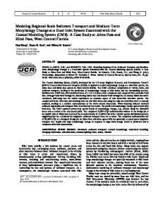
Figure 1. Aerial photograph of steep, soil-mantled landscape, Oregon Coast Range. Note the steep and relatively uniform gradient hillslopes.

Culling [1960, 1963] and Hirano [1968] modeled hillslope evolution through an analogy with Fick’s law of diffusion (in which fluxes are proportional to chemical gradients). In the hillslope analogy, sediment flux (L 3 /L/T) ˜ q s is proportional to the topographic gradient ¹z: q s 5 K lin¹z ˜

(1)

where K lin is linear diffusivity (L 2 /T) and z is elevation (L). Field estimates of downslope sediment flux on low to moderate gradient hillslopes are consistent with (1) over both short [Schumm, 1967] and long [McKean et al., 1993] timescales. Sediment flux and landscape lowering rates can be related through the continuity equation 2r s

z q s 1 r rC o 5 r s¹ ? ˜ t

(2a)

where r r and r s are the bulk densities of rock and sediment, respectively (M/L 3 ), z/t is the rate of change in the land surface elevation (L/T), and C o is the rate of rock uplift (L/T). If the rate of surface erosion is approximately balanced by rock uplift (i.e., dynamic equilibrium, as posited by Gilbert [1909] and Hack [1960]), z/t > 0 and (2a) becomes 2 r rC o 5 r s¹ ? ˜ qs

(2b)

We can combine (1) and (2b) to obtain an expression relating the ratio of the landscape erosion rate (which equals the rock uplift rate C o ) and diffusivity, C o /K lin, and hillslope curvature ¹ 2 z: 2

r rC o 5 ¹ 2z r sK lin

(3)

This relationship indicates that all else being equal, equilibrium hillslopes that erode by linear diffusion should have constant curvature. Recently, geomorphic simulation models have been developed to explore how tectonic activity, climate change, and land use affect landscape evolution [e.g., Nash, 1984; Andrews and Hanks, 1985; Hanks and Schwartz, 1987; Koons, 1989; Willgoose et al., 1991; Rosenbloom and Anderson, 1994; Rinaldo et al., 1995; Arrowsmith et al., 1996; Kooi and Beaumont, 1996; Braun and Sambridge, 1997; Tucker and Slingerland, 1997]. These models simulate hillslope erosion as a linear diffusive process, but the morphology of most soil-mantled hillslopes is inconsistent with the linear diffusion law. Soil-mantled hillslopes typically do not exhibit constant curvature; instead, curvature tends to approach zero as slopes steepen toward a limiting angle (Figure 2). Extreme examples can be found in steep, high-relief mountainous terrain, where many hillslopes are nearly planar, with marked convexity only near divides. This zone of convexity is broader on soil-mantled hillslopes, but there is nonetheless a pronounced decrease in convexity downslope with slopes becoming nearly planar far from the divide. This hillslope form conflicts with constant-curvature (i.e., parabolic) slope profiles predicted by the linear diffusive transport law (Figure 2). What processes could cause this downslope decrease in convexity, and how can such processes be modeled? To simulate the evolution of nearly planar hillslopes, recent landscape evolution models hypothesize that, on steep slopes, sediment transport increases nonlinearly with gradient [Kirkby, 1984, 1985; Anderson and Humphrey, 1989; Anderson, 1994; Howard, 1994a, b, 1997]. These models postulate that sediment


855

discussion of Howard [1997]). These sediment transport models have not been calibrated or directly tested against field data. In this contribution we derive a simple, theoretical expression that describes how sediment transport on soil-mantled hillslopes varies with slope angle. In contrast to previous studies, which have assumed that disturbance-driven transport processes may be represented by linear diffusion, our analysis suggests that diffusive transport varies linearly with slope at low gradients but increases nonlinearly as slope approaches a critical value. We test and calibrate our proposed transport law, using a unique high-resolution topographic data set obtained by airborne laser altimetry. At our study site, hillslope morphology is consistent with our proposed nonlinear diffusion law. Our results indicate that on soil-mantled hillslopes, small changes in slope angle may lead to disproportionate changes in erosion rate.

2. Theory: Nonlinear Diffusive Sediment Transport On soil-mantled hillslopes, disturbances (such as tree throw, animal burrowing, rainsplash, and wet/dry cycles) mobilize sediment, allowing it to be transported downslope. The balance between local frictional and gravitational forces acts to dissipate the energy supplied by disturbances [e.g., van Burkalow, 1945; Jaeger and Nagel, 1992] and may control how sediment flux varies with hillslope angle. Here we present a derivation showing that the combined effects of disturbances, friction, and gravity produce a nonlinear relationship between sediment flux and hillslope gradient. First, we write a general statement for sediment flux (L 3 /L/T) as ˜ qs 5

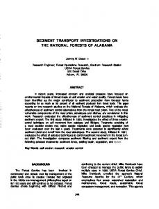
Figure 2. (a) Elevation, (b) gradient, and (c) curvature along a profile for (1) a theoretical hillslope modeled with linear diffusion (equation (1)), shown by thick lines, (2) a hillslope in the Oregon Coast Range (OCR), shown with gray points, and (3) a theoretical hillslope modeled with our proposed nonlinear model (equation (8)), shown by a thin line. The theoretical hillslopes are calculated assuming constant erosion. For both model simulations the diffusivity equals 0.003 m2/yr, the constant erosion rate C o equals 0.075 mm/yr, and r r / r s equals 2.0. For the nonlinear hillslope, S c 5 1.2.

flux combines two distinct process types: (1) diffusive processes (e.g., biogenic activity, rainsplash, soil creep, and solifluction) typically represented with equation (1) and (2) slope failure processes (e.g., soil slips and slumps) which occur more frequently on steep slopes and may be influenced by a threshold slope angle. According to these models, at low slopes, sediment flux increases approximately linearly with gradient, but as slopes approach a critical value, slope failure processes become more prevalent, and small increases in hillslope gradient cause large increases in sediment flux. At or just below this critical gradient, sediment flux is effectively infinite, such that steeper slopes cannot be maintained. As a result, nearly planar hillslopes may evolve, limited by the critical hillslope angle (see

V ˜ v A

(4)

where V/A is the volume of mobile sediment per unit area v is the velocity of its movement along the slope (L 3 /L 2 ) and ˜ downslope (L/T). We assume that over geomorphic timescales, disturbance processes expend energy at a given rate (i.e., supply power) in detaching and mobilizing sediment. Using the physical relationship P 5 Fv ˜; where P is work done in transporting soil per unit time by disturbing agents and F is the net force resisting transport, we can substitute for velocity in (4) and express sediment flux as a function of power per unit area P/A and dissipative force per unit volume F/V: qs 5 ˜

P/A F/V

(5)

In the absence of evidence suggesting a directional preference to disturbance processes, we assume that geomorphic disturbances supply power isotropically on hillslopes, such that equal power is available to move sediment in all directions. The net downslope sediment flux then becomes the difference between the fluxes in the downslope and upslope directions, according to ˜ qs 5

S D P/A F/V

2 down

S D P/A F/V

5 up

P A

S

1 1 2 ~F/V! down ~F/V! up

D

(6)

The upslope and downslope fluxes differ because the downslope dissipative force (F/V) down is less than the upslope dissipative force (F/V) up. Downslope transport is resisted by fric-

856


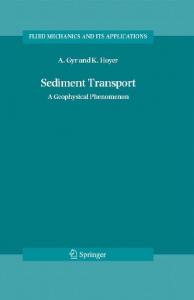
Figure 3. Theoretical relationships between sediment flux and gradient. (curve a) Nonlinear transport law (equation (8)); (line b) linear diffusion law (equation (1)). The critical gradient S c is the gradient at which flux becomes infinite for the nonlinear transport law. tional force (F/V) f and aided by gravitational force (F/V) g , whereas upslope transport is resisted by both friction and gravity, thus (F/V) down 5 (F/V) f 2 (F/V) g , and (F/V) up 5 (F/V) f 1 (F/V) g . For this formulation we assume that friction is the only component of shear strength in the soil. The frictional force per unit volume calculated along the slope is mr s g cos u, and the downslope component of the gravitational force per unit volume is r s g sin u, where m is the effective coefficient of friction, r s is the bulk density of sediment, g is gravitational force, and u is slope angle. The net downslope sediment flux calculated in the horizontal plane then becomes ˜ qs 5

P A

S

2

cos u ~ mr sg cos u 1 r sg sin u !

cos u ~ mr sg cos u 2 r sg sin u !

D

(7)

where the cos u term in the numerator projects the along-slope forces into the horizontal plane. Equation (7) can be simplified. By substituting K 5 (P/A)(2/g m 2 r s ), ¹z 5 tan u, and S c [ m , we obtain a theoretical expression for how sediment flux varies with hillslope gradient: qs 5 ˜

K ¹z 1 2 ~u¹zu/S c! 2

(8)

where K is diffusivity (L 2 /T) and S c is the critical hillslope gradient. In our proposed model, diffusivity varies linearly with the power per unit area supplied by disturbance processes. Diffusivity K also varies inversely to the square of the effective coefficient of friction, m, which follows the intuition that sediment mobilization and transport will vary with the shear strength of the soil. Thus, all else being equal, sediments with more frictional resistance will have lower diffusivities. Andrews and Bucknam [1987] derived a model effectively equivalent to (8), using a framework in which ballistic particles are projected along a hillslope [Hanks and Andrews, 1989]. The behavior of (8) is similar to the transport law proposed

by Howard [1994a, b, 1997] in that sediment flux increases in a nearly linear fashion at low hillslope gradients (which is supported by a field study [McKean et al., 1993]) and increases rapidly as the gradient approaches a critical value (Figure 3) (note: the transport law presented by Howard [1994a, equation (6)] was misprinted; see Howard [1997, equation (2)] for the correct form). In our proposed model the rate of sediment flux becomes infinite at the critical hillslope gradient S c . This attribute of the model is consistent with the concept of threshold hillslopes; when slope angles approach the critical value, increases in the rate of downcutting do not significantly steepen slopes, but instead lead to higher sediment fluxes. We distinguish the critical gradient parameter S c contained in this model from the commonly used “threshold” slope or gradient S t . Assuming that erosion does not become weathering-limited, slope angles equal to S c should not be observable in the field because flux is infinite for such slopes and they would rapidly decline. In contrast, the threshold slope angle is generally equated with the angle of repose and thus is the maximum angle observed in the field [e.g., Strahler, 1950; Carson and Petley, 1970; Young, 1972; Burbank et al., 1996]. Our formulation is not sensitive to the assumption of isotropic power expenditure by diffusive agents. On steep slopes, where power may be preferentially supplied in the downhill direction (i.e., anisotropically), the resulting sediment flux is similar to that predicted by assuming isotropic power expenditure because the net flux is dominated by the downslope component. Our model does not explicitly include small soil slips (which travel short distances over divergent or planar hillslopes) as part of its conceptual framework, but it may capture their diffusive behavior over long timescales. However, our transport law does not address larger landslides that (1) are controlled by elevated pore pressures due to topographically induced convergent subsurface flow, (2) tend to travel long distances through low-order channel networks, (3) scour col-


857

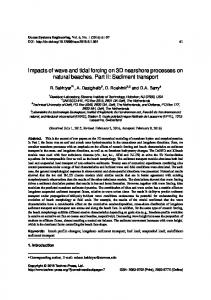
Figure 4. Shaded relief map of study area. Topographic data were obtained with airborne laser altimetry at an average spacing of 2.3 m. The small basins analyzed here are outlined (MR1 5 1, MR2 5 2, MR3 5 3, MR4 5 4, and MR5 5 5). luvium and sediments and expose bedrock, and (4) tend to incise into hillslopes rather than diffuse sediment across them. In the following sections, we describe our study site in the Oregon Coast Range, test the proposed transport law, and describe two techniques for calibrating K and S c . We also compare our proposed transport law with the linear diffusion law and explore its implications for hillslope evolution.

3. 3.1.

Study Site: Oregon Coast Range Description

We tested and calibrated our proposed transport law at five small watersheds within a 2 km2 area of the central Oregon Coast Range (OCR), near Coos Bay, Oregon (Figure 4) (see Montgomery et al. [1997] for location map). We selected this study area because erosion rates are well-documented for small and large spatial scales. Also, at this site, high-resolution topographic data accurately reveal the morphologic signature of diffusive processes. The OCR is a humid, forested, mountainous landscape. Its central and southern regions are underlain by a thick section of Eocene turbidites mapped as the Tyee Formation [Baldwin, 1956; Snavely et al., 1964; Lovell, 1969; Chan and Dott, 1983; Heller et al., 1985]. The Tyee (or sometimes referred to as the Flournoy Formation) has been compressed into a series of low-amplitude, north-northeast striking folds that rarely exhibit dip angles greater than 208 [Baldwin, 1956]. The Oregon Coast Range is situated above a subduction zone and has experienced uplift over the last 20 –30 Myr [Orr et al., 1992]. The topography of the Oregon Coast Range is variable, but significant portions are characterized by steep, highly dissected terrain with distinct ridge and valley topography (Figure 4) [Dietrich and Dunne, 1978; Montgomery, 1991; Montgomery and Dietrich, 1992]. Thin soils typically mantle ridges, and thick colluvial deposits fill unchanneled valleys at the uppermost extent of the channel network. Debris flows originating in unchanneled valleys may control the dissection of low-order channel networks, as fluvial erosion is infrequent in these areas [Dietrich and Dunne, 1978; Swanson et al., 1982; Reneau and Dietrich, 1990; Seidl and Dietrich, 1992]. Diffusive processes

along sideslopes, ridges, and noses transport sediment to unchanneled valleys, where it accumulates until it is removed by landsliding. The probability of landsliding increases with soil depth; thus the rate of sediment supply from adjacent hillslopes controls the timescale of cyclic sediment accumulation and evacuation in hollows [Reneau et al., 1989]. In some locales, inactive deep-seated landslides dominate the topography, having transformed ridge/valley sequences into lowgradient, relatively undissected hillslopes. These massive landslides commonly have a downslope orientation coincident with the downdip direction of the local bedrock, and appear to be concentrated in areas with high dip magnitudes of the underlying bedrock [Roering et al., 1996]. The transport law we propose here applies to purely slope-dependent transport processes on divergent and planar hillslopes, but does not encompass debris flow processes or deep-seated landsliding. The uniformity of highly dissected topography in the Oregon Coast Range suggests that locally, erosion rates may be spatially uniform. Using data from studies of long-term hillslope erosion and short-term, basinwide sediment yield, Reneau and Dietrich [1991] argued that denudation rates (approximately 0.06 – 0.1 mm/yr) in the central Oregon Coast Range do not vary significantly with spatial scale, such that the landscape may be in approximate equilibrium. These denudation rates are also consistent with rates of exfoliation in colluvial bedrock hollows [Reneau and Dietrich, 1991]. Subsequent studies have estimated rock uplift rates as ranging from 0.03 to 0.23 mm/yr in the central Oregon Coast Range [Kelsey and Bockheim, 1994; Kelsey et al., 1994]. By dating strath terraces along many Oregon Coast Range rivers, Personius [1995] estimated similar uplift rates of 0.1– 0.2 mm/yr. More recently, cosmogenic radionuclides have been applied to estimate long-term rates of erosion and soil production, which are 0.1 6 0.03 mm/yr in a small basin within our study site [Heimsath et al., 1996]. The similarity in estimated rates of erosion and uplift suggests approximate equilibrium conditions. However, variability in tectonic and climatic processes may affect rates of channel incision, thereby altering the boundary conditions that drive hillslope erosion. Fernandes and Dietrich [1997] studied the time required for diffusion-dominated hillslopes to establish

858


Plate 1. Topographic maps with the spatial distribution of (a) gradient and (b) curvature for the watershed (MR1) outlined in Figure 4. The contour interval is 2 m. The valley network drains to the north. Positive curvature indicates convergent topography, whereas negative curvature corresponds to divergent terrain. Low-gradient ridges and noses are highly divergent, and hillslopes become steeper and more planar downslope.


859

Figure 5. Theoretical relationships between curvature and gradient generated by three generalized diffusive sediment transport laws (assuming a constant erosion rate C o ). (line a) A linear diffusion law gives hillslopes with constant curvature; (line b) a linear diffusion law coupled with a slope threshold S t , such that steeper slope angles are instantaneously reduced, generates hillslopes with constant curvature below the threshold and planar hillslopes for slopes at the threshold; and (curve c) a nonlinear diffusion law (equation (8)) generates hillslopes with curvature that approaches zero with increasing gradient. Curvature becomes zero when gradient equals the critical value S c .

approximate equilibrium following a change in the channel incision rate. According to their analysis, hillslopes similar to those in our study area would require 150,000 years to reach approximate equilibrium after a doubling of the channel incision rate (exact equilibrium is approached asymptotically). By contrast, the OCR has been uplifting for the last 20 million years [Orr et al., 1992]. These observations suggest that portions of the Oregon Coast Range may approximate an equilibrium landscape, such that over time the terrain erodes at approximately the same rate and rock uplift balances denudation. In other words, the topography of the region may be considered relatively timeindependent (see Howard [1988] for discussion). Despite these observations supporting equilibrium, we observe local features, such as ancient deep-seated landslides, that may indicate local erosional disequilibrium. In performing the analyses described below, we focus on five small watersheds with well-defined divides and relatively uniform ridge and valley morphology because these areas may be more likely to approximate an equilibrium landscape. 3.2. High-Resolution Topographic Data: Airborne Laser Altimetry In our study area, high-resolution topographic data were obtained using airborne laser altimetry (Airborne Laser Mapping, Inc.), which can accurately characterize fine-scale topographic features over large areas [e.g., Garvin, 1994; Ritchie et al., 1994; Armstrong et al., 1996; Ridgway et al., 1997]. Topographic data points were collected with an average spacing of 2.3 m and a vertical resolution of approximately 0.2– 0.3 m. In addition to depicting fundamental geomorphic features, such as ridges and unchanneled valleys, and anthropogenic features, such as logging roads and landings, the topographic data provide a detailed description of meter-scale irregularities on hillslopes (see Figure 4). The expression of small-scale roughness presumably reflects data errors in distinguishing vegetation

from the ground surface, as well as the stochastic nature of tree throw pits and local lithologic variability.

4. Characterizing Sediment Transport Laws With Topographic Derivatives 4.1.

Method

We used plots of hillslope curvature as a function of gradient (e.g., Figures 5 and 6) to test diffusive transport laws against the hillslope morphology of our study site. Most landscape evolution models employ one of three general relationships for how sediment flux varies with slope. Each of these three general transport laws generates a distinct relationship between hillslope gradient and curvature for equilibrium hillslopes (Figure 5). First, the linear diffusive transport law (equation (1)) implies that on equilibrium hillslopes, curvature does not vary with gradient (see equation (3)). Second, some studies have suggested that hillslopes denude by linear diffusion unless a threshold angle S t is attained [e.g., Ahnert, 1976; Avouac, 1993; Tucker and Slingerland, 1994; Arrowsmith et al., 1996]. Upon reaching the threshold angle, hillslopes experience an immediate downslope redistribution of sediment (i.e., landslide). Equilibrium hillslopes modeled with such a transport law would exhibit constant curvature for gradients below the threshold and be planar (zero curvature) for gradients at or near the threshold. Thus plots of curvature versus gradient would approximate a step function at the threshold slope angle (see Figure 5). Finally, nonlinear transport laws (e.g., equation (8)) imply that hillslope curvature should be roughly constant at low gradients, converging continuously toward zero with increasing gradient (see Figure 5). Curvature equals zero for gradients equal to the critical value S c . Using the relationship between hillslope gradient and curvature, we can assess the validity of the three generalized sediment transport laws. Traditionally, hillslope profiles have been used to analyze

860


Figure 6. (a– e) Plot of gradient against curvature for our study basins (MR1–MR5) and (f) moving downslope along individual hillslopes in MR1–MR4. Open diamonds indicate binned average values of curvature. Low-gradient terrain tends to be convex (highly negative curvature), whereas steep terrain tends to be nearly planar (near zero curvature). The relationship is consistent with our nonlinear transport law (see Figure 5), such that curvature decreases continuously with gradient and approaches zero for steep slopes.

the morphologic expression of sediment transport laws [e.g., Davis, 1892; Penck, 1953; King, 1963; Kirkby, 1971; Howard, 1994a, b], as we show in Figure 2. Profiles are a simple and appealing method for describing slope morphology, but they cannot account for planform (i.e., contour) curvature. In our study site, as well as in many soil-mantled landscapes, hillslope segments with negligible planform curvature are rare, confounding our ability to characterize hillslope morphology with profiles. Alternatively, plots of gradient against curvature (calculated in both the x and y directions) allow us to directly compare hillslope form to models of hillslope erosion. Using this approach, we can test these models across large areas, rather than restricting our analysis to selected hillslope profiles. We estimated topographic gradient and curvature by fitting two-dimensional, second-degree polynomials to patches of local topographic data points (300 –500 m2) at evenly spaced intervals throughout the study basins. We used a weighted least squares routine (which gives greater weight to points near the center of each patch) and calculated gradient and curvature

from the coefficients of the best fit equations. Our analysis is based on laser altimetry-derived topographic data that captures meter-scale variability in the topography. Topographic data obtained from digital elevation models with a large grid spacing (e.g., 30 m or larger) will not accurately depict smallscale variations in hillslope morphology that are indicative of most diffusive processes. 4.2.

Results

Plate 1 depicts a small catchment (MR1, which is approximately 52,000 m2) with characteristic ridges and valleys in our study site near Coos Bay, Oregon. The spatial distribution of gradient (u¹zu) and curvature (calculated as the Laplacian operator ¹ 2 z) delineates the structure of ridges and valleys. Ridges (which are narrow, divergent hilltops that extend over long distances) and noses (which are divergent hillslopes with unchanneled valleys on either side) tend to have divergent (highly negative ¹ 2 z) axes and high gradient, nearly planar (near zero ¹ 2 z) sideslopes. Noses alternate with convergent (highly positive ¹ 2 z) unchanneled valleys. Curvature appears


to decrease gradually as one moves in the downslope direction from hilltops. To quantify hillslope morphology and assess the sediment transport laws discussed above, we plotted gradient against curvature for hillslopes (which we defined as areas with ¹ 2 z , 0) in the five small basins depicted in Figure 4. Low-gradient portions of hillslopes tend to be highly divergent, whereas steep sideslopes typically have near zero values of curvature. In each of our study basins, we observe a gradual trend toward zero curvature with increasing gradient (Figures 6a– 6e), which indicates that the topography is consistent with our nonlinear diffusive transport law (equation (8)). Moving downslope along individual hillslopes in these basins, we also observe the trend of decreasing convexity with increasing gradient (Figure 6f). More generally, we observe that (1) curvature is not constant and (2) an abrupt threshold slope angle does not separate low-gradient, divergent slopes from steep, planar slopes. Thus the morphologic signature depicted in Figure 6 is fundamentally inconsistent with both the linear diffusion law and the linear diffusion/slope threshold law.

5. Model Calibration: Divergence of Sediment Flux 5.1.

Method

Our calibration procedure finds the values of K and S c that are most consistent with the topographic form of our study area and its measured long-term erosion rate. We calculate erosion rate E as the divergence of sediment transport, E 5 ¹ z˜ q s . Substituting (8), we obtain the following expression that relates the rate of landscape erosion to model parameters (K and S c ) and derivatives of the local topographic field:

E5

2K r r/ r s 2 1

3

¹ 2z 1 2 ~u¹zu/S c! 2

FS D z x

2

S D

S

DG4

2z z 2 2z z z 2z 21 21 2 x y y y x xy S2c ~1 2 ~u¹zu/Sc !2 !2

(9)

From (9) and assumed values for K and S c , we can calculate the local erosion rates of individual points on the landscape from their topographic derivatives. If the landscape is in steady state, then each point on the landscape should be eroding at the same rate. Our calibration procedure searches for the values of K and S c that make these modeled erosion rates as uniform as possible across the landscape, and as consistent as possible with independently derived estimates of the long-term average erosion rate C o . We limited our analysis to divergent or nearly planar hillslopes (i.e., ¹ 2 z , 0) because our sediment transport model (equation (8)) does not address masswasting processes associated with convergent topography. The calibrated or best fit parameters are those that minimize the difference between modeled erosion rates (equation (9)) and the assumed long-term erosion rate C o . For the calibration we used a constant landscape erosion rate C o of 0.1 6 0.03 mm/yr [Heimsath et al., 1996] and r r / r s 5 2.0 6 0.2 [Reneau and Dietrich, 1991]. We plot the root mean square error (RMSE) between C o and modeled erosion rates for a range of values of K and S c , and choose the parameters that give the lowest value of RMSE:

RMSE 5

F

1 n

O n

~C o 2 E i!

2

i51

861

G

1/ 2

(10)

where n is the number of points in the landscape for which we model the erosion rate and E i is the modeled erosion rate at the ith point in the landscape (calculated with equation (9)). The vertical resolution of topographic data may affect our results. To estimate how uncertainty in the elevation (i.e., z) values affects our calibrated parameters, we performed a Monte Carlo simulation. Specifically, we randomly varied the elevation values within their range of uncertainty and recalibrated the model parameters from this “synthetic” data set. By performing many iterations of this process, we estimated the probability distribution and standard error of the calibrated model parameters. 5.2.

Results

We performed the calibration on five small basins in our study area (see Figure 4). For catchment MR1 we plotted RMSE (normalized by C o ) as a function of K and S c and found the minimum value of RMSE/C o (approximately 0.4) when K 5 0.0032 6 0.0009 m2/yr and S c 5 1.25 6 0.10 (Figure 7). Calibrated parameters for all five study basins are shown in Table 1. Values for K range from 0.0031 to 0.0045 m2/yr with an average of 0.0036 m2/yr, and S c ranges from 1.2 to 1.35 with an average value of 1.27. Thus the variability of the parameter estimates between our five small basins is consistent with our estimate of the parameter uncertainty within each individual basin. The shape of the surface defining RMSE/C o in Figure 7, which dips steeply in either direction parallel to the K axis and dips less steeply parallel to the S c axis, indicates that the model calibration is more sensitive to variability in K than in S c . Diffusivity K is linearly related to the spatially constant landscape erosion rate, such that any adjustments in C o give proportional changes in K. Recalibrating the model parameters in our Monte Carlo simulation, we observed that our results are relatively insensitive to uncertainty in the topographic data. For example, our calculations show that the standard error in K due to topographic uncertainty is approximately 0.0001 m2/yr and for S c it is approximately 0.02. Thus topographic uncertainty is a small part of the total uncertainty in estimates of K and S c .

6. 6.1.

Model Calibration: Area Slope Method

We can also calibrate the model parameters by modeling sediment fluxes using (8) and comparing them to the sediment fluxes required to maintain a spatially uniform erosion rate. This method tests our proposed model more directly, although it does not define the estimated parameters as precisely as the divergence method. In an equilibrium landscape the volumetric sediment flux per unit length across each point is qs 5 Co

rr a rs b

(11)

where a/b is drainage area per unit contour length. We plot mass flux (equation (11)) as a function of hillslope gradient and estimate K and S c by fitting theoretical flux curves (equation (8)) to the data points.

862


Figure 7. Contour plot of RMSE/C o as a function of K and S c for basin MR1. The surface defines the misfit, according to equation (10), between modeled erosion rates and the spatially constant rate (0.1 mm/yr) for different parameter values. The lowest value of RMSE/C o , as shown by the gray lines, corresponds to the best fit parameters (K 5 0.0032 m2/yr, and S c 5 1.25). Contours with extremely high values of RMSE/C o were omitted for clarity. Analogous to Gilbert’s [1909] conceptual model of a onedimensional hillslope, (11) states that mass flux must increase with drainage area on equilibrium hillslopes. If sediment transport varies primarily with gradient (as we hypothesize for divergent and planar hillslopes), points with higher a/b should also have steeper hillslope gradients. To restrict this analysis to hillslopes, we limited our calculations to points of the landscape with negative curvature. Generally, these points have a/b values below a particular threshold, such that higher values tend to be associated with convergent topography (e.g., hollows and channels) [Tarboton et al., 1991; Dietrich et al., 1992; Montgomery and Foufoula-Georgiou, 1993]. To calculate a/b, we used a grid-based analysis and applied a multidirection, weighted-area algorithm that uses the grid node spacing as b (similar to Costa-Cabral and Burges [1994] and Tarboton Table 1. Calibrated Parameters Using Divergence Calibration Method in Study Basins Site MR1 MR2 MR3 MR4 MR5 Average

K, m2/yr

Sc

0.0032 0.0031 0.0045 0.0032 0.0039

1.25 1.20 1.35 1.35 1.22

0.0036 6 0.0016

1.27 6 0.16

[1997]). In this calculation the total area draining out of each grid cell is divided between its downslope neighbors (both adjacent and diagonal) in proportion to the local gradient. This algorithm produces a spatial distribution of a/b that avoids obvious grid artifacts that would be created if the maximum fall line were used to calculate drainage area. 6.2.

Results

On hillslopes in catchment MR1, a/b increases with gradient, which is consistent with the equilibrium assumption, such that points with larger drainage areas must transmit higher mass fluxes (Figure 8). However, for convergent parts of the landscape, a/b varies inversely with gradient; these points are part of the valley network and thus are not included in the model calibration. In catchment MR1 we observe that flux (calculated with equation (11) for points in the landscape with negative curvature) increases nearly linearly with gradient for low slopes and increases rapidly on steeper slopes (Figure 9). To calibrate the model parameters, we fit two model flux curves (equation (8)) to the data, such that over 98% of the data points are enclosed by the two curves. These curves define a range of model parameters; K varies between 0.0015 and 0.0045 m2/yr, and S c varies between 1.0 and 1.4. These parameters define the bounds of values consistent with our study basin and are similar to parameter values estimated with the divergence method (K 5 0.0032 m2/yr, and S c 5 1.25). For very low gradients (,0.2), mass flux estimates exceed those pre-


863

Figure 8. Semilog plot showing the relationship between drainage area per unit contour length (a/b) and gradient for basin MR1 (see Plate 1). Black dots represent terrain with divergent curvature (which we classify as hillslopes), and gray dots represent convergent terrain. Values are calculated from gridded topography with a 4 m spacing, thus the smallest possible value of a/b equals 4 m. dicted by the model because cells in our simulation have a finite size (4 3 4 m) and smaller drainage areas cannot be computed.

7.

Modeling Hillslope Morphology

To analyze how our proposed transport law influences hillslope morphology, we calculated how erosion rate affects gradient and curvature along an equilibrium model hillslope. Specifically, we solved (9) in one dimension assuming a constant erosion rate C o and using the calibrated value of S c 5 1.25. We used this simple, one-dimensional analysis because twodimensional hillslope evolution modeling requires the specification and calibration of transport laws for valley-forming processes such as debris flows and fluvial erosion (those endeavors exceed the scope of this contribution). Figure 10 depicts gradient (Figure 10a) and curvature (Figure 10b) as a function of distance from the divide (L) for a range of r r C o / r s K. Figure 10 shows that for slope gradients greater than roughly 0.5 S c , large increases in erosion rate can be accommodated by small increases in hillslope gradient. For example, 25 m downslope of the divide, only a 25% increase in gradient (from 0.75 to 0.97) is required to accommodate a doubling of the erosion rate (from r r C o / r s K equals 0.05 to 0.10 m21). With increasing distance from the divide, hillslope gradient becomes increasingly uniform, and both slope and curvature become increasingly insensitive to changes in erosion rate. Using calibrated

values of K and S c , we plotted model curves against the hillslope profile depicted in Figure 2 (which had negligible planform curvature) to demonstrate that nonlinear diffusive transport is more appropriate for representing the observed hillslope morphology than linear diffusion. For very low values of r r C o / r s K (,0.01 m21), the modeled hillslope has relatively constant curvature and approximates a hillslope modeled with linear diffusion. In other words, when erosion rates are low relative to diffusivity, hillslope gradients will not approach the critical slope S c except on very long hillslopes. With increasing erosion rate (or decreasing diffusivity), the point along the hillslope at which curvature deviates from a constant value moves closer to the divide. For extremely high values of r r C o / r s K, slope angles increase rapidly downhill of the divide and approach a threshold value such that lower sections of the hillslope are steep and nearly planar. More generally, with increasing erosion rate, decreasing diffusivity, and increasing hillslope length, more of the hillslope will be close to the critical angle.

8.

Observed and Modeled Hillslope Morphology

To explore how nonlinear diffusion may affect hillslope morphology, we plotted the frequency distribution of hillslope gradient in our study catchments, and compared it to the slope dependence of sediment flux (as estimated from equation (8)).

864


Figure 9. Relationship between sediment flux and gradient in basin MR1. Data points indicate flux computed with equation (11), which is calculated for parcels of the landscape with divergent curvature. Two model curves, which are computed with equation (8), are plotted around the data points, such that over 98% of the data points are enclosed by the two curves. The dashed curve has K 5 0.0015 m2/yr, and S c 5 1.4; the solid gray curve has K 5 0.0045 m2/yr, and S c 5 1.0. Flux does not approach zero (or fit within the model curves) because a finite grid cell size limits the smallest possible value of a/b.

In our study basins, ridges and noses typically bisect steep sideslopes; on these sideslopes, angles approach and sometimes exceed 458. The scale of the highly convex region is of the order of 10 m, and the average hillslope length is approximately 35 m; thus a large fraction of the hillslope area lies outside the highly convex region and instead is steep and nearly planar. We plotted our calibrated sediment transport law (K 5 0.0032 m2/yr, and S c 5 1.25) and the frequency distribution of gradient for hillslopes in MR1–MR5 (Figure 11a). In our study basins, hillslope gradients tend to cluster near values for which sediment flux is a highly nonlinear function of slope (for example, in MR1, mean hillslope gradient is 0.80, and 50% of the terrain has gradients between 0.74 and 0.92). Sediment flux increases rapidly with gradient near the critical slope; this feedback results in a limit to slope steepness. To test the observed clustering of gradients near the nonlinearity in mass flux, we compared the gradient distributions for MR1–MR5 (see Figure 11a) with the gradient distribution for an equilibrium, one-dimensional, model hillslope (Figure 11b). This simple, one-dimensional analysis captures how our transport law influences the distribution of hillslope gradient and curvature. We modeled the equilibrium hillslope with the following parameters: K 5 0.0032 m2/yr, S c 5 1.25, C o 5 0.1 mm/yr, r r / r s 5 2.0, and hillslope length is equal to 35 m. Hillslope gradients for the study basins and model hillslope are similarly clustered between 0.7 and 1.0, although the model hillslope has more area with lower gradients, between 0 and 0.6. This discrepancy arises because our theoretical hillslope

must have zero slope at the divide, whereas divides in our study basins are typically inclined along their axes; thus slopes in the study basins tend to be steeper. In addition, some hillslopes in our study basins have significant planform curvature, which further diminishes the area with low gradient (i.e., ridges). We also compared the cumulative distribution of curvature for MR1–MR5 and the theoretical hillslope (Figure 12). These distributions illustrate that the majority of hillslope area has curvature between 0 and 20.04.

9. Modeling Erosion Rates: Linear and Nonlinear Diffusive Transport Laws To evaluate how our proposed transport law compares with linear diffusion for modeling erosion rates at our study site, we calculated the frequency distribution of erosion rate using both laws. In both cases, we calculated erosion rates at evenly spaced points on divergent terrain in basin MR1. For the nonlinear case we used (9) (with the calibrated parameters K 5 0.0032 m2/yr, and S c 5 1.25) and plotted the frequency distribution of the calculated erosion rates (Figure 13). For the linear model we used (10) to calibrate (1) and found the value of K lin that minimizes the misfit between modeled erosion rates and the spatially constant value C o 5 0.1 mm/yr. We used the best fit K lin (approximately 0.0053 m2/yr) to model erosion rates with (1) and (2a) and plotted the frequency distribution of calculated erosion rates (Figure 13). From this analysis we observe that neither transport law


10.

Figure 10. Contour plot of hillslope (a) gradient and (b) curvature as a function of the ratio of erosion rate to diffusivity (C o /K) and hillslope length L for an equilibrium hillslope modeled in one dimension with equation (9) (S c 5 1.25).

generates a uniform erosion rate. In fact, both models indicate that local erosion rates vary between 0 and over 0.16 mm/yr. Despite this variability, our nonlinear model produces a cluster of values around the assumed constant erosion rate of 0.1 mm/yr. The linear model generates more low erosion rates because erosion is proportional to curvature and our study site is dominated by nearly planar hillslopes. For the nonlinear model, over 70% of the study site has a modeled erosion rate between 0.05 and 0.15 mm/yr, whereas for the linear model, less than 40% of the terrain has a modeled erosion rate in that range. This result suggests that the proposed nonlinear transport law would better preserve the current topography than would the linear law. In other words, denudation modeled by the linear model would substantially alter hillslope morphology, rounding sideslopes and producing a wider distribution of gradient. The nonlinear model is more consistent with steady state erosion given the observed hillslope morphology.

865

Discussion

Our analysis yields a nonlinear diffusive transport law that is consistent with the tendency of hillslopes in our study area to become more planar as they steepen. Our transport law behaves similarly to those proposed by Kirkby [1984, 1985], Anderson [1994], and Howard [1994a, b, 1997] in that flux increases continuously with gradient and increases rapidly as gradients approach a critical value. Although these models have sometimes been termed “landslide” laws, we refer to (8) as a nonlinear diffusive transport law because our proposed model does not encompass large landslides or debris flows and does not require them to produce the observed nonlinear slope dependence of sediment flux. Transport laws that attempt to represent debris flows should include a mechanism to account for the area dependency of pore pressure development, such that convergent areas experience more frequent soil saturation and thus have a higher probability of generating a shallow landslide [Tucker and Bras, 1998]. Our proposed transport law differs from those discussed above because it suggests that purely diffusive processes, such as biogenic activity, generate a nonlinear relationship between hillslope gradient and sediment flux. Kirkby [1984, 1985], Anderson [1994], and Howard [1994a, b, 1997] suggest that a process transition occurs on steeper slopes, such that slope failure processes become more prevalent and cause a rapid increase in flux with gradient. Because the critical gradient term S c imposes a condition of chronic soil instability in our model, we suggest that it may effectively encompass small soil slips and slumps that do not travel far, although these processes are not explicitly included in the theoretical formulation. Sediment transport rates predicted with our proposed model are similar to those obtained by field studies. Reneau and Dietrich [1991] estimated colluvial transport rates by defining sideslope pathways of sediment transport into hollows and measuring the amount of colluvium deposited above dated organic material. The average colluvial transport rate for nine sites in the southern Oregon Coast Range is 0.0032 6 0.0023 m2/yr. Most of the sideslopes in their study area have a relatively uniform slope angle, and the average value was measured for each site. To test (8) against the transport rates measured by Reneau and Dietrich [1991], we calculated sediment flux (or colluvial transport rate) using our calibrated model and the average gradient of sideslopes in their study (approximately 0.7). Our model predicts a colluvial transport rate of approximately 0.0036 m2/yr, which is similar to their average value of 0.0032 m2/yr. Using their average colluvial transport rate and the average sideslope gradient, we calculated an average linear diffusivity K lin which is approximately 0.0048 m2/yr. This value is very similar to the calibrated value of K lin (0.0053 m2/yr) that we estimated using the equilibrium assumption and topographic data. Estimated values of K lin are larger than estimates of K because of the nonlinearity in our proposed flux relationship (equation (8)). For a given diffusivity our proposed transport law predicts higher sediment fluxes for gradients near the critical value than does the linear diffusion law. We suggest that steep, soil-mantled landscapes may be appropriately modeled with a nonlinear diffusive transport law because (1) the topography of our study site is consistent with a nonlinear diffusive transport law and (2) our calibrated model generates rates of mass flux similar to those measured in the field. Our topographic analyses (Figures 6 and 9) and erosion rate

866


Figure 11. Calibrated relationship between flux and gradient (shown by dashed curve, with K 5 0.0032 m2/yr, and S c 5 1.25) and the frequency distribution of hillslope gradients (shown with solid curves) for (a) our study basins and (b) a one-dimensional, equilibrium hillslope modeled with equation (8) (K 5 0.0032 m2/yr, and S c 5 1.25). Gradient distributions reveal a clustering between 0.7 and 1.0.

calculations (Figure 13) suggest that the morphology of our study basins is consistent with an approximate equilibrium landscape eroding by nonlinear diffusive processes. Although hillslope convexity tends to decrease with gradient (as our model predicts), we observe significant variance in this trend, which may indicate that some locales are eroding faster or slower than our assumed constant value C o . Similarly, we observe a tendency for modeled erosion rates to cluster around our assumed constant value (C o 5 0.1 mm/yr), but portions of basin MR1 have modeled erosion rates that are not within 50% of C o . These observations suggest that local deviations from equilibrium may exist in our study basins. These deviations may reflect hillslope response to changing boundary conditions or the influence of variable rock properties. Through our model calibration, we estimated the critical gradient to be approximately 1.25 (or 518). This value exceeds the internal friction angle of most soils, suggesting that cohesion from roots or other sources contributes shear strength to soils in our study area. We suggest that S c may effectively

represent the total shear strength of the soil, although the model formulation does not explicitly account for shear strength from sources other than granular friction. Our estimate of S c is somewhat scale-dependent because slopes may be even steeper locally (e.g., within a pit/mound feature). Nonetheless, field measurements of slope angle generally agree with calculations from the digital topographic data, and rarely did we observe slope angles exceeding 458–508 in the field. Our analysis assumes that soil depth does not affect the rate of sediment transport on hillslopes. Ahnert [1967, 1976] hypothesized that sediment flux may vary nonlinearly with soil depth, such that equilibrium hillslopes may be planar with soil depth increasing downslope. He suggested that shear stresses generated at the base of a soil column may cause the soil to deform or flow [e.g., Fleming and Johnson, 1975]. In our study area we observe an easily distinguishable boundary between colluvium, which is typically coarse-grained and rich in organic material, and weathered bedrock or saprolite. On ridges,


Figure 12. Plot of cumulative percentage of divergent terrain for our study basins and for a one-dimensional, equilibrium hillslope modeled with equation (8). The majority of curvature values for both the study site and the theoretical hillslope are between 20.04 and 0.0. noses, and sideslopes, soil depth ranges between about 0.2 and 1.0 m and does not covary with curvature, slope angle, or distance downslope (K. M. Schmidt, manuscript in preparation, 1998; A. M. Heimsath et al., manuscript in preparation, 1998), suggesting that sediment flux does not vary systematically with soil depth. The stochastic nature of diffusive processes, such as tree throw and mammal burrowing, leads to large variability in local soil depth. We argue that soil depth may not affect sediment flux in our study area because the soils are coarse; frictional resistance would prevent significant shearing or flowing. Instead, soils are transported by periodic disturbances, which overcome the frictional resistance of the colluvium and the shear strength provided by root cohesion. Our proposed model applies only to the transport of soil, thus diffusive transport rates are limited by soil production rates if bedrock slopes emerge. Our topographic analysis and model calibration procedures assume that rates of soil production are sufficient to maintain soil-mantled hillslopes, and this

867

assumption is consistent with our field observations. If erosion rates exceed rates of soil production, hillslopes may be stripped of their soil mantle, and different erosional processes may become dominant, such as rock fall, rock toppling, and other forms of bedrock landsliding [e.g., Howard and Selby, 1994]. Heimsath et al. [1997] suggest that biogenic processes control the rate of soil production, which decreases exponentially with soil depth. Climatic and biogenic variability, whether natural or anthropogenic, may influence the soil production function defined by Heimsath et al. [1997], although these relationships have been unexplored. Previous field and experimental studies have reported results that are consistent with a nonlinear diffusion transport law. Strahler [1950, p. 673] analyzed hillslopes in southern California and found a uniformity of slope angle that he attributed to “a prevailing condition of form-equilibrium.” Lithology, climate, soil, vegetation, and channel location were used to distinguish slopes in different stages of development. In his analysis, Strahler [1950] noted that hillslopes with channels actively incising at their base tended to exhibit the steepest slope angles, which tended to cluster around a value similar to the angle of repose. Furthermore, gentler slopes were associated with creep processes and were distinct from those controlled by a limiting slope angle. Several hillslope profiles from Strahler [1950] showed distinctly convex hilltops with increasingly planar slopes downhill, such that creep and landsliding may combine to generate the observed hillslope morphology. Experimental studies of rainsplash are consistent with our nonlinear model. For a given rainfall rate, measurements of rainsplash creep, which is defined as sediment transport by raindrop impact, demonstrate a nonlinear increase in creep rate with increasing gradient [Moeyersons, 1975]. In addition, Moeyersons [1975] reported that flux rates are linearly related to rainfall rate. This finding is consistent with our proposed theoretical model in that power is linearly related to sediment flux, if we consider rainfall rate as a measure of the power responsible for mobilizing and transporting sediment (see equation (8)). In an experimental study of sediment transport by rainsplash, Mosley [1973] quantified flux as a function of gradient, although he did not report results for slopes greater

Figure 13. Frequency distribution of modeled erosion rates in basin MR1 for calibrated linear (shown by thin dashed curve, equation (1)) and nonlinear (thick gray curve, equation (8)) transport laws. Both transport laws were calibrated assuming a constant erosion rate of 0.1 mm/yr (equation (10)). For the nonlinear transport law, K equals 0.0032 m2/yr, and S c 5 1.25, whereas for the linear diffusion law, K lin 5 0.0053 m2/yr.

868


than 258 because “rolling and sliding of grains” became prevalent. Such behavior may be consistent with our proposed transport law in that rapid increases in flux occur on steep slopes. Diffusion models depend on measures of topographic curvature, which depend on the resolution of the underlying topographic data. Many studies that use linear diffusion (equation (1)) to explore large-scale landscape evolution are based on topographic data with coarse resolution (30 –1000 m) and assume that “scaled-up” transport laws can appropriately represent geomorphic processes at scales larger than their scale of occurrence, as discussed by Anderson and Humphrey [1989] and Koons [1989]. In the Oregon Coast Range, diffusive processes operate over length scales of only a few meters or less, as is typical of soil-mantled landscapes. The analyses reported here are possible because of the availability of high-resolution topographic data. Alternative approaches have been proposed for simulating rapid increases in flux at high gradients. For example, Martin and Church [1997] used historical landslide data to define different diffusivities for high and low gradient hillslopes. The high-gradient diffusivity represents “rapid, episodic mass movements.” Also, many models of landscape evolution and fault scarp evolution couple a linear diffusion law and a threshold slope angle, such that higher angles are instantaneously reduced to the threshold value [e.g., Ahnert, 1976; Avouac, 1993; Tucker and Slingerland, 1994; Arrowsmith et al., 1996]. As opposed to these coupled models, nonlinear transport laws predict that a rapid (but continuous) increase in sediment transport can be used to approximate the development of threshold slopes [Howard, 1997]. Our topographic analysis (see Figure 6) demonstrates that a continuous transport function may be more appropriate than slope thresholds for modeling the erosion of steep, soil-mantled hillslopes. Previous studies propose that hillslope gradient is influenced by rates of valley incision and may reflect threshold hillslope processes. Through their analysis of river incision rates and digital topographic data along a swath of terrain in the northwestern Himalayas, Burbank et al. [1996] conclude that the average angle of hillslopes is steep and independent of erosion rate, such that landsliding allows for hillslopes to adjust efficiently to river downcutting. Schmidt and Montgomery [1995] suggest that bedrock landsliding results from a combination of slope and local relief, such that the maximum hillslope angle varies with the elevation difference between ridges and valley bottoms. Howard [1997] provided insight on thresholdcontrolled erosional regimes through a landscape evolution model. In exploring relationships between erosion rate, relief, and drainage density, he states “in steep terrain, erosion rates may be sufficiently high that slope gradient is generally close to failure conditions z z z slope gradient then becomes essentially independent of erosion rate or location on the slope” [Howard, 1997, p. 215]. In our study basins, hillslope gradients are sufficiently close to the critical value to generate the behavior that Howard [1997] describes. The mean gradient for these hillslopes is approximately 0.80 (or 65% of the critical slope), and over 80% of gradients exceed 0.6. Slight increases in slope angle should generate large increases in mass flux, and slope angles may be limited by this feedback; for a given channel spacing, local relief therefore may be largely independent of erosion rate. Our analysis suggests that rates of uplift or erosion may not be easily discerned from hillslope steepness [e.g., Kelsey et al.,

1994; Summerfield and Nulton, 1994; Aalto and Dunne, 1996; Granger et al., 1996]. Near the critical slope, large changes in erosion rates are associated with only slight changes in hillslope gradient, so the topographic signature of tectonic forcing will be small. Although changes in erosion rate have only a small effect on average gradient, they will cause proportional changes in hillslope curvature near hilltops and divides (see Figure 10). Thus the topographic signature of tectonic forcing may more clearly be found in hilltop curvature rather than in sideslope gradient. If the diffusivity K can be estimated independently, hilltop curvature can be used as a quantitative measure of erosion rate. Because slopes become more planar with distance from the divide, curvature can be more precisely estimated (and will be more clearly related to erosion rate) close to divides and hilltops.

11.

Conclusion

In steep, soil-mantled landscapes, the interaction between diffusive processes and shallow landsliding is reflected in alternating sequences of ridges and unchanneled valleys. Hillslope sediment transport processes influence not only the evolution of hillslope morphology, but also the rates of hollow infilling and evacuation by debris flows, the rates of sediment flux into channel networks, and the distribution of soil on hillslopes. We modeled diffusive sediment transport and its implications for hillslope morphology. Our conclusions from this analysis are as follows: 1. Diffusive sediment transport has traditionally been modeled as a linear function of gradient (equation (1)). Our theoretical analysis shows that diffusive processes should produce a nonlinear relationship between sediment flux and slope (equation (8)). This analysis yields a nonlinear diffusive transport law in which sediment flux increases nearly linearly for shallow gradients, but increases rapidly as gradient approaches a critical slope angle (Figure 3). 2. At our study site, hillslopes tend to become increasingly planar with increasing gradient, consistent with our proposed nonlinear transport law (Plate 1 and Figure 6). Hillslope morphology at our study site is inconsistent with linear diffusion. 3. We calibrated our nonlinear transport law using highresolution topographic data for our study site (Figure 4). This calibration assumes that the local terrain used in our analysis is in approximate erosional steady state. Our calibrated parameters yield sediment transport rates that are consistent with field estimates obtained by measuring colluvial deposition rates in hollows. Topographic modeling of erosion rates shows a clustering around the estimated constant value. However, modeled erosion rates for 30% of our study area differ by more than 50% of the assumed constant value, suggesting that the equilibrium assumption may only be approximately met. 4. With increasing erosion rate, decreasing diffusivity, and increasing hillslope length, our proposed model predicts that hillslopes should become steeper and increasingly planar. 5. In our study site, hillslope gradients tend to cluster near values for which sediment flux is a highly nonlinear function of gradient (0.7– 0.9), such that slope angles may be limited by large increases in mass flux at high gradients. Because slight variations in hillslope gradient may correspond to a large variations in erosion rate, slope angle will not be a sensitive indicator of tectonic forcing. The signature of tectonic forcing will be more reliably manifested in the topographic curvature of hilltops and divides.

ROERING ET AL.: EVIDENCE FOR NONLINEAR, DIFFUSIVE SEDIMENT TRANSPORT Acknowledgments. This work was funded through NSF grant EAR-9357931 to J.W.K. The authors thank A. Heimsath, A. Howard, C. Riebe, K. Schmidt, L. Sklar, and J. Stock for insightful discussions. We also thank T. Hanks, R. Iverson, and D. Montgomery for thorough and thoughtful reviews that greatly improved the manuscript.

References Aalto, R. E., and T. Dunne, Geomorphic controls of Andean denudation rates, Eos Trans. AGU, 77(46), Fall Meet. Suppl., 245, 1996. Ahnert, F., The role of the equilibrium concept in the interpretation of landforms of fluvial erosion and deposition, in L’evolution des Versants, edited by P. Macar, pp. 23– 41, Univ. of Liege, Liege, France, 1967. Ahnert, F., Brief description of a comprehensive three-dimensional process-response model of landform development, Z. Geomorphol. Suppl., 25, 29 – 49, 1976. Anderson, R. S., Evolution of the Santa Cruz Mountains, California, through tectonic growth and geomorphic decay, J. Geophys. Res., 99, 20,161–20,174, 1994. Anderson, R. S., and N. F. Humphrey, Interaction of weathering and transport processes in the evolution of arid landscapes, in Quantitative Dynamic Stratigraphy, edited by T. A. Cross, pp. 349 –361, Prentice-Hall, Englewood Cliffs, N. J., 1989. Andrews, D. J., and R. C. Bucknam, Fitting degradation of shoreline scarps by a nonlinear diffusion model, J. Geophys. Res., 92, 12,857– 12,867, 1987. Andrews, D. J., and T. C. Hanks, Scarp degraded by linear diffusion; inverse solution for age, J. Geophys. Res., 90, 10,193–10,208, 1985. Armstrong, E. M., J. C. Brock, M. W. Evans, W. B. Krabill, R. Swift, and S. S. Manizade, Beach morphology in the southeastern United States from airborne laser altimetry, Eos Trans. AGU, 77(46), Fall Meet. Suppl., 393, 1996. Arrowsmith, J. R., D. D. Pollard, and D. D. Rhodes, Hillslope development in areas of active tectonics, J. Geophys. Res., 101, 6255– 6275, 1996. Avouac, J.-P., Analysis of scarp profiles: Evaluation of errors in morphological dating, J. Geophys. Res., 98, 6745– 6754, 1993. Baldwin, E. M., Geologic map of the lower Siuslaw River area, Oregon, U.S. Geol. Surv. Oil Gas Invest. Map, OM-186, 1956. Benda, L., and T. Dunne, Stochastic forcing of sediment supply to channel networks from landsliding and debris flow, Water Resour. Res., 33, 2849 –2863, 1997. Black, T. A., and D. R. Montgomery, Sediment transport by burrowing animals, Marin County, California, Earth Surf. Processes Landforms, 16, 163–172, 1991. Braun, J., and M. Sambridge, Modeling landscape evolution on geological time scales; a new method based on irregular spatial discretization, Basin Res., 9, 27–52, 1997. Burbank, D. W., J. Leland, E. Fielding, R. S. Anderson, N. Brozovic, M. R. Reid, and C. Duncan, Bedrock incision, rock uplift and threshold hillslopes in the northwestern Himalayas, Nature, 379, 505–510, 1996. Carson, M. A., and M. J. Kirkby, Hillslope Form and Process, 475 pp., Cambridge Univ. Press, New York, 1972. Carson, M. A., and D. J. Petley, The existence of threshold hillslopes in the denudation of the landscape, Trans. Inst. Br. Geogr., 49, 71–95, 1970. Chan, M. A., and J. Dott, Shelf and deep-sea sedimentation in Eocene forearc basin, Western Oregon-fan or non-fan?, Am. Assoc. Petrol. Geol. Bull., 67, 2100 –2116, 1983. Costa-Cabral, M. C., and S. J. Burges, Digital elevation model networks (DEMON): A model of flow over hillslopes for computation of contributing and dispersal areas, Water Resour. Res., 30, 1681– 1692, 1994. Culling, W. E. H., Analytical theory of erosion, J. Geol., 68, 336 –344, 1960. Culling, W. E. H., Soil creep and the development of hillside slopes, J. Geol., 71, 127–161, 1963. Davis, W. M., The convex profile of badland divides, Science, 20, 245, 1892. Dietrich, W. E., and T. Dunne, Sediment budget for a small catchment in mountainous terrain, Z. Geomorphol. Suppl., 29, 191–206, 1978. Dietrich, W. E., S. L. Reneau, and C. J. Wilson, Overview; “zero-order basins” and problems of drainage density, sediment transport and hillslope morphology, in Erosion and Sedimentation in the Pacific

869

Rim, vol. 165, edited by R. L. Beschta et al., pp. 27–37, Int. Assoc. of Hydrol. Sci., Corvallis, Oreg., 1987. Dietrich, W. E., C. J. Wilson, D. R. Montgomery, J. McKean, and R. Bauer, Erosion thresholds and land surface morphology, Geology, 20, 675– 679, 1992. Dietrich, W. E., R. Reiss, M.-L. Hsu, and D. R. Montgomery, A process-based model for colluvial soil depth and shallow landsliding using digital elevation data, Hydrol. Processes, 9, 383– 400, 1995. Fernandes, N., and W. E. Dietrich, Hillslope evolution by diffusive processes: The timescale for equilibrium adjustments, Water Resour. Res., 33, 1307–1318, 1997. Fleming, R. W., and A. M. Johnson, Rates of seasonal creep of silty clay soil, Q. J. Eng. Geol., 8, 1–29, 1975. Garvin, J. B., Topographic characterization and monitoring of volcanoes via airborne laser altimetry, in Volcano Instability on the Earth and Other Planets, vol. 110, edited by W. J. McGuire, A. P. Jones, and J. Neuberg, pp. 137–152, Geol. Soc. London, London, 1994. Gilbert, G. K., The convexity of hilltops, J. Geol., 17, 344 –350, 1909. Granger, D. E., J. W. Kirchner, and R. Finkel, Spatially averaged long-term erosion rates measured from in-situ produced cosmogenic nuclides in alluvial sediment, J. Geol., 104, 249 –257, 1996. Hack, J. T., Interpretation of erosional topography in humid temperate regions, Am. J. Sci., 258A, 80 –97, 1960. Hack, J. T., and J. C. Goodlett, Geomorphology and forest ecology of a mountain region in the central Appalachians, U.S. Geol. Surv. Prof. Pap., 347, 66 pp., 1960. Hanks, T. C., and D. J. Andrews, Effect of far-field slope on morphologic dating of scarplike landforms, J. Geophys. Res., 94, 565–573, 1989. Hanks, T. C., and D. P. Schwartz, Morphologic dating of the pre-1983 fault scarp on the Lost River Fault at Doublespring Pass Road, Custer County, Idaho, Bull. Seismol. Soc. Am., 77, 837– 846, 1987. Heimsath, A. M., W. E. Dietrich, K. Nishiizumi, and R. C. Finkel, Soil production and landscape equilibrium: Hillslope analysis using cosmogenic nuclides in Northern California and coastal Oregon, Eos Trans. AGU, 77(46), Fall Meet. Suppl., 245, 1996. Heimsath, A. M., W. E. Dietrich, K. Nishiizumi, and R. C. Finkel, The soil production function and landscape equilibrium, Nature, 388, 358 –361, 1997. Heller, P. L., Z. E. Peterman, J. R. O’Neil, and M. Shafiqullah, Isotopic provenance of sandstones from the Eocene Tyee Formation, Oregon Coast Range, Geol. Soc. Am. Bull., 96, 770 –780, 1985. Hirano, M., A mathematical model of slope development—An approach to the analytical theory of erosional topography, J. Geosci., 11, 13–52, 1968. Howard, A. D., Equilibrium models in geomorphology, in Modelling Geomorphological Systems, edited by M. G. Anderson, pp. 49 –72, John Wiley, New York, 1988. Howard, A. D., A detachment-limited model of drainage basin evolution, Water Resour. Res., 30, 2261–2285, 1994a. Howard, A. D., Badlands, in Geomorphology of Desert Environments, edited by A. D. Abrahams and A. J. Parsons, pp. 213–242, Chapman and Hall, New York, 1994b. Howard, A. D., Badland morphology and evolution: Interpretation using a simulation model, Earth Surf. Processes Landforms, 22, 211– 227, 1997. Howard, A. D., and M. J. Selby, Rock slopes, in Geomorphology of Desert Environments, edited by A. D. Abrahams and A. J. Parsons, pp. 123–172, Chapman and Hall, New York, 1994. Hungr, O., A model for the runout analysis of rapid flow slides, debris flows, and avalanches, Can. Geotech. J., 32, 610 – 623, 1995. Iverson, R. M., M. E. Reid, and R. G. LaHusen, Debris-flow mobilization from landslides, Ann. Rev. Earth Planet. Sci., 25, 85–138, 1997. Jaeger, H. M., and S. R. Nagel, Physics of the granular state, Science, 255, 1523–1530, 1992. Johnson, K. A., and N. Sitar, Hydrologic conditions leading to debrisflow initiation, Can. Geotech. J., 27, 789 – 801, 1990. Kelsey, H. M., and J. G. Bockheim, Coastal landscape evolution as a function of eustasy and surface uplift rate, Cascadia margin, southern Oregon, Geol. Soc. Am. Bull., 106, 840 – 854, 1994. Kelsey, H. M., D. C. Engebretson, C. E. Mitchell, and R. L. Ticknor, Topographic form of the Coast Ranges of the Cascadia margin in relation to coastal uplift rates and plate subduction, J. Geophys. Res., 99, 12,245–12,255, 1994. King, L. C., South African Scenery: A Textbook of Geomorphology, 308 pp., Hafner, New York, 1963.

870


Kirkby, M. J., Hillslope process-response models based on the continuity equation, Inst. Br. Geogr. Spec. Publ., 3, 15–30, 1971. Kirkby, M. J., Modeling cliff development in South Wales: Savigear re-reviewed, Z. Geomorphol., 28, 405– 426, 1984. Kirkby, M. J., A model for the evolution of regolith-mantled slopes, in Models in Geomorphology, edited by M. J. Woldenberg, pp. 213–237, Allen and Unwin, Winchester, Mass., 1985. Kooi, H., and C. Beaumont, Large-scale geomorphology: Classical concepts reconciled and integrated with contemporary ideas via a surface processes model, J. Geophys. Res., 101, 3361–3386, 1996. Koons, P. O., The topographic evolution of collisional mountain belts: A numerical look at the Southern Alps, New Zealand, Am. J. Sci., 289, 1041–1069, 1989. Lovell, J. P. B., Tyee Formation: Undeformed turbidites and their lateral equivalents: Mineralogy and paleogeography, Geol. Soc. Am. Bull., 80, 9 –22, 1969. Martin, Y., and M. Church, Diffusion in landscape development models: On the nature of basic transport relations, Earth Surf. Processes Landforms, 22, 273–279, 1997. McKean, J. A., W. E. Dietrich, R. C. Finkel, J. R. Southon, and M. W. Caffee, Quantification of soil production and downslope creep rates from cosmogenic 10Be accumulations on a hillslope profile, Geology, 21, 343–346, 1993. Moeyersons, J., An experimental study of pluvial processes on granite gruss, Catena, 2, 289 –308, 1975. Montgomery, D. R., Channel initiation and landscape evolution, Ph.D. thesis, 421 pp., Univ. of Calif., Berkeley, Berkeley, 1991. Montgomery, D. R., and W. E. Dietrich, Channel initiation and the problem of landscape scale, Science, 255, 826 – 830, 1992. Montgomery, D. R., and E. Foufoula-Georgiou, Channel networks sources representation using digital elevation models, Water Resour. Res., 29, 1925–1934, 1993. Montgomery, D. R., W. E. Dietrich, R. Torres, S. P. Anderson, J. T. Heffner, and K. Loague, Hydrologic response of a steep, unchanneled valley to natural and applied rainfall, Water Resour. Res., 33, 91–109, 1997. Mosley, M. P., Rainsplash and the convexity of badland divides, Z. Geomorphol. Suppl., 18, 10 –25, 1973. Nash, D. B., Morphologic dating of fluvial terrace scarps and fault scarps near West Yellowstone, Montana, Geol. Soc. Am. Bull., 95, 1413–1424, 1984. Orr, E. L., W. N. Orr, and E. M. Baldwin, Geology of Oregon, 254 pp., Kendall/Hunt, Dubuque, 1992. Penck, W., Morphological Analysis of Landforms, 429 pp., Macmillan, Indianapolis, Ind., 1953. Personius, S. F., Late Quaternary stream incision and uplift in the forearc of the Cascadia subduction zone, western Oregon, J. Geophys. Res., 100, 20,193–20,210, 1995. Pierson, T. C., Factors controlling debris-flow initiation on forested hillslopes in the Oregon Coast Range, Ph.D. thesis, 166 pp., Univ. of Wash., Seattle, 1977. Reneau, S. L., and W. E. Dietrich, Depositional history of hollows on steep hillslopes, coastal Oregon and Washington, Natl. Geogr. Res., 6, 220 –230, 1990. Reneau, S. L., and W. E. Dietrich, Erosion rates in the Southern Oregon Coast Range: Evidence for an equilibrium between hillslope erosion and sediment yield, Earth Surf. Processes Landforms, 16, 307–322, 1991. Reneau, S. L., W. E. Dietrich, M. Rubin, D. J. Donahue, and A. J. T. Jull, Analysis of hillslope erosion rates using dated colluvial deposits, J. Geol., 97, 45– 63, 1989. Ridgway, J. R., J. B. Minster, N. Williams, J. L. Bufton, and W. B. Krabill, Airborne laser altimeter survey of Long Valley, California, Geophys. J. Int., 131, 267–280, 1997. Rinaldo, A., W. E. Dietrich, R. Rigon, G. K. Vogel, and I. Rodriguez-

Iturbe, Geomorphological signatures of varying climate, Nature, 374, 632– 635, 1995. Ritchie, J. C., E. H. Grissinger, J. B. Murphey, and J. D. Garbrecht, Measuring channel and gully cross-sections with an airborne laser altimeter, Hydrol. Processes, 8, 237–243, 1994. Roering, J. J., J. W. Kirchner, and W. E. Dietrich, Identification and characterization of deep-seated landslides in the Oregon Coast Range using digital terrain data, Eos Trans. AGU, 77(46), Fall Meet. Suppl., 246, 1996. Rosenbloom, N. A., and R. S. Anderson, Hillslope and channel evolution in a marine terraced landscape, Santa Cruz, California, J. Geophys. Res., 99, 14,013–14,029, 1994. Schmidt, K. M., and D. R. Montgomery, Limits to relief, Science, 270, 617– 620, 1995. Schumm, S. A., Evolution of drainage systems and slopes in badlands at Perth, Amboy, New Jersey, Bull. Geol. Soc. Am., 67, 597– 646, 1956. Schumm, S. A., Rates of surficial rock creep on hillslopes in western Colorado, Science, 155, 560 –562, 1967. Seidl, M. A., and W. E. Dietrich, The problem of channel erosion into bedrock, Catena Suppl., 23, 101–124, 1992. Sidle, R. C., Shallow groundwater fluctuations in unstable hillslopes of coastal Alaska, Z. Gletscherkd. Glazialgeol., 20, 79 –95, 1984. Snavely, P. D., H. C. Wagner, and N. S. MacLeod, Rhythmic-bedded eugeosynclinal deposits of the Tyee Formation, Oregon Coast Range, Kans. Geol. Surv. Bull., 169, 461– 480, 1964. Strahler, A. N., Equilibrium theory of erosional slopes approached by frequency distribution analysis, Am. J. Sci., 248, 673– 696, 1950. Summerfield, M. A., and N. J. Nulton, Natural controls of fluvial denudation rates in major world drainage basin, J. Geophys. Res., 99, 13,871–13,883, 1994. Swanson, F. J., R. L. Fredriksen, and F. M. McCorison, Material transfer in a western Oregon forested watershed, in Analysis of Coniferous Forest Ecosystems in the Western United States, edited by R. L. Edmonds, pp. 233–366, Van Nostrand Reinhold, New York, 1982. Tarboton, D. G., A new method for the determination of flow directions and upslope areas in grid digital elevation models, Water Resour. Res., 33, 309 –319, 1997. Tarboton, D. G., R. L. Bras, and I. Rodriguez-Iturbe, On the extraction of channel networks from digital elevation data, Hydrol. Processes, 5, 81–100, 1991. Tucker, G. E., and R. L. Bras, Hillslope processes, drainage density, and landscape morphology, Water Resour. Res., 34, 2751–2764, 1998. Tucker, G. E., and R. L. Slingerland, Erosional dynamics, flexural isostasy, and long-lived escarpments: A numerical modeling study, J. Geophys. Res., 99, 12,229 –12,243, 1994. Tucker, G. E., and R. L. Slingerland, Drainage basin responses to climate change, Water Resour. Res., 33, 2031–2047, 1997. van Burkalow, A., Angle of repose and angle of sliding friction: An experimental study, Bull. Geol. Soc. Am., 56, 669 –708, 1945. Willgoose, G., R. L. Bras, and I. Rodriguez-Iturbe, Results from a new model of river basin evolution, Earth Surf. Processes Landforms, 16, 237–254, 1991. Young, A., Slopes, in Geomorphology Texts, vol. 3, edited by K. M. Clayton, 288 pp., Oliver and Boyd, White Plains, N. Y., 1972. W. E. Dietrich, J. W. Kirchner, and J. J. Roering (corresponding author), Department of Geology and Geophysics, University of California,Berkeley,Berkeley,CA94720-4767.(e-mail:roering@geomorph. berkeley.edu) (Received May 15, 1998; revised October 22, 1998; accepted November 9, 1998.)

Evidence for nonlinear, diffusive sediment transport on ... - CiteSeerX

Evidence for nonlinear, diffusive sediment transport on ... - CiteSeerX

Suggest Documents

Nonlinear double-diffusive convection - CiteSeerX

Foraminiferal evidence of submarine sediment transport and ...

Relativistic diffusive transport

Evidence for fluvial sediment transport of Kalahari ...

Application of diffusive transport model for better

Two-scale model for electro-diffusive transport

Modeling Regional-Scale Sediment Transport and ... - CiteSeerX

management effects on runoff and sediment transport in ... - CiteSeerX

Hydrology, Hydraulics, and Sediment Transport ... - CiteSeerX

sediment transport investigations on the national forests of ... - CiteSeerX

Sediment Transport Study

SEDIMENT TRANSPORT MECHANISM

1 SEDIMENT TRANSPORT STUDY ON THE ...

Biological influence on sediment transport and bed

Sediment transport through rock groynes on mixed

sediment transport model applicable

SEDIMENT TRANSPORT ON CAPE SABLE, EVERGLADES ...

Sediment Transport

Sediment transport - Infoscience - EPFL

Artificial neural networks for sheet sediment transport - CiteSeerX

Unit stream power for sediment transport in natural rivers ... - CiteSeerX

Dissipative charge transport in diffusive superconducting double ...https://www.researchgate.net/...junctions/.../Dissipative-charge-transport-in-diffusive-s...

ON A CLIMATE MODEL WITH A DYNAMIC NONLINEAR DIFFUSIVE ...

Sediment Transport Formula for Steep Channels