WCCI 2010 IEEE World Congress on Computational Intelligence July, 18-23, 2010 - CCIB, Barcelona, Spain
FUZZ-IEEE
Evolving Fuzzy Optimally Pruned Extreme Learning Machine: A Comparative Analysis Federico Montesino Pouzols, Member, IEEE and Amaury Lendasse, Member, IEEE Abstract— This paper proposes a method for the identification of evolving fuzzy Takagi-Sugeno systems based on the Optimally-Pruned Extreme Learning Machine (OP-ELM) methodology. We describe ELM which is a simple yet accurate and fast learning algorithm for training single-hidden layer feed-forward artificial neural networks (SLFNs) with random hidden neurons. We then describe the OP-ELM methodology for building ELM models in a robust and generic manner. Leveraging on the previously proposed Online Sequential ELM method and the OP-ELM, we propose an identification method for self-developing or evolving neuro-fuzzy systems. This method follows a random projection based approach to extracting evolving fuzzy rulebases. A comparison is performed over a diverse collection of datasets against well known evolving neuro-fuzzy methods, namely DENFIS and eTS. It is shown that the method proposed is robust and competitive in terms of accuracy and speed.
I. I NTRODUCTION Evolving, online or adaptive intelligent systems are meant to be applied on sequential data or streams of data. These systems distinguish themselves from traditional, offline learning methods and previous online methods in that their structure (in addition to their parameters) evolves in order to account for new data. The interest in self-developing artificial neural network methods can be tracked back to some early works in the field [1]. During the last decade there has been an increase of interest in this field and in particular within the area of evolving fuzzy systems for modeling and control [2]. Some recent advances include DENFIS [3], and the more general Evolving Connectionist Systems framework [4], and evolving Takagi-Sugeno (eTS) [5] as well as its variants [6]. For instance, evolving TS fuzzy systems [5] combine supervised and unsupervised learning techniques to evolve the TS model structure as well as its parameters as new data become available. This way, new rules can be added, existing rules can be reorganized, and in general any aspect of an evolving fuzzy inference model is subject to selfdevelopment. Evolving fuzzy systems represent a relative recent step beyond the paradigms of self-tunning neuro-fuzzy systems [7] and online neuro-fuzzy systems [5]. In general, the evolving approach implies the need for simple, one-pass training methods as opposed to traditional, iterative algorithms. Evolving Federico Montesino Pouzols and Amaury Lendasse are with the Department of Information and Computer Science, Aalto University School of Science and Technology, P.O. Box 15400, FI-00076 Aalto, Espoo, Finland (phone: +358-9-470-25237; email:
[email protected],
[email protected]). FMP is supported by a Marie Curie Intra-European Fellowship for Career Development (grant agreement PIEF-GA-2009237450) within the European Community´s Seventh Framework Programme (FP7/2007–2013).
c 978-1-4244-8126-2/10/$26.00 2010 IEEE
fuzzy systems are particularly useful for online prediction and predictive control. Among other advantages, evolving fuzzy systems provide an inherent capability for novelty detection and an enhanced robustness against nonstationarities. This paper proposes a method for the identification of evolving fuzzy Takagi-Sugeno systems based on the Optimally-Pruned Extreme Learning Machine (OP-ELM) methodology. We leverage in three previous developments: the ELM learning method, introduced by Huang et al. [8], the OP-ELM methodology, introduced by Miche et al. [9], and the online sequential ELM algorithm, introduced by Liang et al. [10] and extended for fuzzy systems by Rong et al. [11]. ELM challenges conventional learning methods and theories. ELM has been shown to be accurate and fast both theoretically and experimentally. Indeed, ELM is extremely fast but can achieve a performance in terms of generalization comparable to other accurate yet costly learning techniques. OP-ELM has been introduced by Miche et al. [9] in order to improve the robustness of ELM models. This is achieved through a three stages methodology which includes steps for fast ranking of hidden neurons and model selection. Rong et al. [11] have previously shown that single hiddenlayer feedforward neural networks (SLFNs) can be regarded as equivalent to fuzzy inference systems. They use this equvalence in order to derive an online sequential method for fuzzy systems (OS-Fuzzy-ELM) based on the online sequential ELM [10]. Here we introduce an evolving approach to the identification of evolving Takagi-Sugeno fuzzy inference systems based on the original offline OP-ELM methodology and the OS-ELM online learning algorithm. We exploit the equivalence between SLFNs and FIS, and bring the good performance and robustness of the OP-ELM methodology together with the online approach of OS-ELM in order to define the evolving fuzzy OP-ELM (eF-OP-ELM). The paper is organized as follows. Section II describes the ELM, the OP-ELM methodology and the OS-ELM sequential learning algorithm. In section III we introduce the evolving fuzzy OP-ELM (eF-OP-ELM) modeling approach for building evolving fuzzy inference systems. Then, in section IV a comparative analysis is performed against other well-known alternatives. Section V discusses results with an emphasis on the interpretability achieved through the OP-ELM model selection scheme. Finally we give some concluding remarks. II. ELM The Extreme Learning Machine (ELM) [8], [12] is a simple yet effective learning algorithm for training single-
1339
hidden-layer feed-forward artificial neural networks (SLFNs) with random hidden nodes. In ELM, the hidden neuron parameters are randomly assigned whereas the output weights are analytically determined. ELM is a unified framework of generalized SLFNs that has the universal approximation capability for a wide range of hidden node types. The training process for ELM can be several orders of magnitude faster than traditional learning algorithms for feed-forward neural networks, while attaining similar or even better approximation capabilities. Let us consider a dataset consisting of M observations (xj , yj ) ∈ Rd1 × Rd2 , being d1 the dimension of the input space and d2 the dimension of the output space. An SLFN with N neurons in the hidden layer is defined by the following expression: N X
βi f (xj , ci , ai ),
1 ≤ j ≤ M,
i=1
where f (·) is the activation function and βi ∈ R are the output weights. Let us illustrate two widely studied architectures of SLFNs: SFLNs with hidden additive nodes and radial basis function (RBF) networks which use RBF nodes in the hidden layer. Additive nodes have the form f (ci · xj + bi ), where wj ∈ Rd1 are the input weights and bi x −c the biases. RBFs have the form f (|| jbi i ||), where wj ∈ Rd1 are the centers and bi the widths of the RBF nodes. If the SFLN perfectly fits the data, then the difference ˆ i and the actual output values between the estimated outputs y is zero and thus the following holds: N X
β i f (xj , ci , ai ) = yj ,
1 ≤ j ≤ M,
i=1
which can be written as: Hβ = Y, with
f (x1 , c1 , a1 ) .. H= . f (xM , c1 , a1 )
... .. . ...
(1) f (x1 , cN , aN ) .. , . f (xM , cN , aN )
T T T β = (β1T , . . . , βN ) and Y = (y1T , . . . , yM ) . In the ELM method, the hidden layer, H, is generated in in a random way, independenly of the training dataset. Then, the output weights of the SLFN, β can be determined analytically. The estimated output weights are computed as:
ˆ = H† Y, β
(2)
where H† is the Moore-Penrose generalized inverse of H. For the applicable implementation methods refer to [10], [8]. As pointed out by Huang [13] the ELM theory claims that parameter tuning is not required. This approach challenges conventional learning methods and theories. It has been theoretically shown that for function approximation all the parameters of the hidden nodes can be randomly generated without any prior knowledge. In [8]
it is proved that the hidden-layer output matrix can be computed (and achieves an approximation error as small as desired) for N ≤ M , under the assumption that the activation function is infinitely differentiable. The universal approximation capability of ELM has been proved in [12]. This way, ELM is a extremely fast method [8], several orders of magnitude faster than traditional feedforward neural networks methods while competitive in terms of accuracy. As a final remark, ELM only requires the number of neurons in the hidden layer to be specified, as opposed to other learning methods which often have several hyperparameters to be tuned. A. Optimally-Pruned ELM (OP-ELM) The Optimally Pruned Extreme Learning Machine (OPELM) models [9], [14], [15] is a methodology based on the ELM. OP-ELM models are built in three stages and use Gaussian, sigmoid and linear kernels in general. First, an ELM is constructed, then, an exact ranking of the neurons in the hidden layer is performed, and finally the decision on how many neurons are pruned is made based on an exact leaveone-out error estimation method. These stages are performed by means of fast methods and lead to extremely fast yet accurate models. OP-ELM has been shown to provide a compromise between the speed of ELM and the accuracy and robustness of other much more computationally intensive methods. OPELM models achieve roughly the same level of accuracy as that of other well known computational intelligence methods [9], [14], such as Support Vector Machines and Least Squares Support Vector Machines [16], Gaussian Processes and Multilayer Perceptrons [17], while being significantly faster. As explained above, only one parameter has to be tuned in order to build accurate ELM models: the number of hidden neurons. In principle the only feasible approaches to a sensible tuning of the number of hidden neurons are based on the definition of validation subsets. This is the approach used generally in the literature [8], [10]. However, validation approaches such as cross-validation and bootstrapping methods raise several issues. In particular, computational cost increases significantly, which is specially troublesome for online, adaptive and possibly realtime systems. In addition, validation methods assume the different subsets used for training, validation and test are drawn from the same population. For systems that evolve or exhibit nonstationarity, whether statistical or dynamical, this assumption may lead to wrong models. The OP-ELM method introduced a sound approach to the selection of the subset of best nodes in such a way that unuseful neurons are pruned. This brings in a fundamental advantage for evolving methods besides enhancing the robustness of ELM models against irrelevant and redundant variables [9]. In what follows we outline the 3 stages of the OP-ELM methodology. 1) Construction of an initial SLFN: This step is performed using the standard ELM algorithm for a large enough
1340
number of neurons N 1 . 2) Ranking of Hidden Neurons: The Multiresponse Sparse Regression (MRSR) [19] algorithm is applied in order to rank the hidden neurons according to their accuracy. MRSR is in essence a generalization of the least angle regression (LARS) algorithm, and is thus able to find an exact ranking for linear problems. Since in a ELM model the output is linear with respect to the randomly initialized hidden nodes, the MRSR ranking within the OP-ELM methodology is exact. This way, the variables for the MRSR algorithm, hi (the outputs of the hidden nodes or columns of the hidden node matrix, H), are ranked exactly by their performance. 3) Model Selection: Once a ranking of the the kernel has been obtained. the best number of neurons for the model has to be chosen. Methods based on offline validation, such as leave-one-out are often used for this kind of task. They can be however extremely expensive in computational terms and quickly become unaffordable for large datasets or online, evolving or time constrained systems. However, the LOO can be directly calculated for linear models by using the PRESS (PREdiction Sum of Squares) statistics, which provides the following closed-form expression for the LOO error of linear models: RESS εP = i
yi − hi bi , 1 − hi PhTi
where i denotes the ith hidden node, and P is defined as P = (HT H)−1 , being H the hidden layer output matrix. The optimal number of neurons can be found by estimating the LOO error for different numbers of nodes (already ranked by accuracy) and selecting the number of neurons L such that minimizes the error: L = argmin
j X
j∈{1,...,N } i=1
RESS εP i
(3)
It has been shown that the ranking (previous) stage of the OPELM method has two positive effects: convergence is faster and the number of neurons required to achieve the lowest LOO error is lower [9]. B. Online Sequential ELM (OS-ELM) The original ELM method is designed for offline modeling. However thanks to the simplicity of the computations in the ELM method, it is possible to define efficient online extensions for ELM. Liang et al. [10] have proposed the OS-ELM algorithm which we outline in this section for the purposes of providing all the equations used in the next section. The algorithm first computes a standard ELM model for an initialization training set, with output matrix Y0 , hidden nodes matrix H0 , and solution β (0) = (HT0 H0 )−1 HT0 Y0 , using the Moore-Penrose generalized inversion according to 2. Let us define K0 = HT0 H0 . Then, for each new 1 By default the initial number of neurons used in the OP-ELM Toolbox [18], [14] is 100.
observation or chunk of observations the model is updated online by means of the following recursive expressions: β (k+1) = β (k) + Pk+1 HTk+1 (Yk+1 − Hk+1 β k ),
(4)
Pk+1 = Pk − Pk HTk+1 (I + Hk+1 Pk HTk+1 )−1 Hk+1 Pk , (5) where Pk+1 = K−1 k+1 . These recursive update rules are obtained by using the Sherman-Morrison-Woodbury formula for computing the inverse of a rank-k correction of matrices. We refer to [10] for the full details. III. E VOLVING F UZZY OP-ELM The rules of a Takagi-Sugeno (TS) fuzzy inference model, applied to a certain input xj , can be generally expressed as [5]: Ri : IF(xj1 is Ai1 ) AND . . . AND (xjd1 is Aid1 ), THEN (yj1 is βi1 ) . . . (yjd2 is βid2 ), where d1 is the dimension of the input space, d2 is the dimension of the output space, i = 1, . . . , L for a rulebase consisting of L rules, and Aik , (k = 1, . . . , d1 ; i = 1, . . . , L) are the fuzzy sets for the kth input variable xj in the ith rule. βik (k = 1, . . . , d2 ; i = 1, . . . , L) are crisp values, linear combinations of the input variables in the form βik = qik,0 + qik,1 x1 + . . . + qik,d1 xd1 for a first-order TS model. For each fuzzy set, Aik , the degree of membership of a given input xj is specified by its corresponding membership function µAik (xj ). A nonconstant piecewise continuous membership function f (c, a) can be considered as in [11]. This kind of function includes most common membership functions such as Gaussian and triangular as well as virtually all practical possibilities. The membership function can thus be defined by any bounded nonconstant piecewise continuous membership function as follows: µAik (xj ; cki , ai ) = f (xj ; cki , ai ), where ak and cjk are the parameters of the membership function f (·) for the ith rule and the kth component of the input vectors, xj . In a fuzzy inference system of this type, the output of the model is computed as the weighted sum of the output of each rule, where the weights are the activation degrees of the ˆ j for an input xj is given as rules. Thus, the system output y follows: PL L X i=1 β i Ri (xj ; ci , ai ) ˆj = P β i f (x; , ci , ai ), = y L i=1 Ri (xj ; ci , ai ) i=1
(6)
where β i = (βi1 , . . . , βim ), and f (·) can be seen as a normalized rule: Ri (xj ; ci , ai ) . (7) f (xj ; , ci , ai ) = PL i=1 Ri (xj ; ci , ai ) According to the equivalence between generalized SFLN and FIS, Rong. et al. have established the interpretation of
1341
OS-ELM as an online fuzzy model [11] applicable to both regression and classification problems. As noted in [11] f as expressed in (7) is what can be called a fuzzy basis function (FBF) [20]. In (6) it is evident that a FIS is equivalent to a generalized SLFN, where f (·) represents the output functions of the hidden layer and β represents the output weight vector. This way, the output functions of the hidden nodes of the SLFN are equivalent to the FBFs of the FIS, which in turn are based on the membership functions. Note this equivalence is used in [11] to develop an online method for the identification of fuzzy inference systems of the Takagi-Sugeno type (OS-Fuzzy-ELM). Note though that this method is online (as OS-ELM [10]) yet not fully evolving, i.e., the system self-tunes in an online manner but the system structure (rulebase) does not evolve. As a particular case of fuzzy or neuro-fuzzy system, an evolving TS fuzzy system can be represented as a neural network [21]. We show in what follows how to generalize for an online learning approach the following two elements in the OP-ELM methodology: the LARS-based ranking process, and the PRESS statistics-based estimation of the LOO error. Following the equivalence betwen the structure of SFLN and FIS, the latter can be expressed in terms of the former: F(xj ) =
L X
β i f (xj ; ci , ai ) = tj ,
(8)
i=1
for a certain number of rules L. In the TS type models the consequent of each fuzzy rule is a linear equation of the input variables. If the coefficients, qik,j , k = 1 . . . d2 , j = 1 . . . d1 , of the linear equations are arranged in a matrix of parameters of the model for the ith rule as follows: qi1,0 . . . qid2 ,0 .. .. .. qi = , . . . qi1,d1
...
qid2 ,d1
then β i = xTje qi , where xje = [1, xTje ]T is obtained by appending a 1 to the input vector in order to generate a linear equation. This way, expanding β in 8, the output of the model can be expressed as follows: F(xj ) =
L X
xTje qi f (xj ; ci , ai ) = yj ,
j = 1, . . . , M.
i=1
The above expression in compact form is: HQ = Y, which is a generalization of (1), with: q1 Q = ... . qL Since a TS FIS is equivalent to an SLFN, the ELM learning method can be applied to a fuzzy system. Thus, given that H is initialized randomly and Y is known, Q can be computed
online using the same approach as in OS-ELM, as developed in [11] for OS-Fuzzy-ELM. In the evolving fuzzy OP-ELM (eF-OP-ELM), the output of the TS model is as follows: L(j)
F(j, xj ) =
X
xTie qi (j)f (xj , ci (j), ai (j)) = yj ,
(9)
i=1
which in compact form can be expressed as: H(j)Q(j) = Y(j),
j ≥ 1,
for xj being the last observation available. Here, H(j) is an evolving matrix, i.e., L(j) (the number of rules or nodes in the hidden layer of the equivalent ELM) can evolve as well as the input membership functions and the consequent parameters. In this method the rulebase is fully evolving and thus the hidden nodes matrix takes the following form: f (xk , c1 (j), a1 (j)) . . . f (xk , cL(j) (j), aL (j)) .. .. .. H(j) = , . . . f (xj , c1 (j), a1 (j)) . . . f (xj , cL(j) (j), aL (j)) where 1 ≤ k ≤ j, L(j) is the evolving number of rules, ci (j) ∈ C and ai (j) ∈ A are the parameters of the input membership functions, and C and A are sets of parameters values generated randomly in the initizalization stage. Putting all pieces together, we can describe how the components of an evolving TS fuzzy inference system are defined in the eF-OP-ELM method: • The antecedents (or “IF” part) belong to a set of antecedents that is created randomly by generating the sets of parameters C and A. • The concrete subset of rules are selected as in the 2nd and 3rd stages of the OP-ELM methodology. • The corresponding consequents (or “THEN” part) are generated analytically using the ELM method, according to (2). The eF-OP-ELM algorithm consists of the following steps: Algorithm 1 Evolving Fuzzy OP-ELM (eF-OP-ELM) 1: A set of antecedents is created randomly by generating the sets of parameters C and A, of cardinality N . 2: For a given initialization dataset consisting of M observations (xj , yj ) ∈ Rd1 × Rd2 , an M -by-N matrix of hidden nodes, H0 (j), j = M, is generated by applying the fuzzy basis functions as in (7). 3: The fuzzy rules in H0 (j) are ranked and the best number of rules are selected (as in (3)) following the OPELM methodology. The result, H(j), j = M , allows for the computation of Q(j), j = M, (as in (2)). The initial evolving TS model, F(·), is generated with the form of (9). 4: When a new observation, xj , becomes available: 4.1: Update H0 (j) with the new observation and apply the 2nd and 3rd stage of the OP-ELM methodology in order to generate the evolving H(j). 4.2 Find the analytical solution for Q(j). The model output at time j can now be computed.
1342
TABLE I DATASETS : NUMBER OF INPUTS , TRAINING OBSERVATIONS AND TEST
IV. E XPERIMENTS
OBSERVATIONS
Dataset Abalone Auto-MPG Bank Breast Cancer Delta Ailerons Servo Stocks Mackey-Glass Santa Fe Laser ENSO Sunspots Darwin SLP Internet2
# Inputs 8 7 8 32 5 4 9 4 3 3 7 5 4
Training length 2784 258 3000 129 4752 111 633 500 988 465 2085 904 708
Test length 1393 134 1500 65 2377 56 317 9093 400 1000 467 730
with time step 0.1 s for the following differential equation: x(t) ˙ =
0.2x(t − τ ) − 0.1x(t). 1 + x10 (t − τ )
The initial conditions and delay parameter are x(0) = 1.2, x(t) = 0 for t < 0, τ = 17, and the value of the series 85 steps ahead (x(t + 85)) has to be modeled based on 4 inputs: x(t), x(t − 6), x(t − 12) and x(t − 18). Refer to [3] for the full details required to generate the dataset. In order to replicate the subseries of 500 values used in [5], the values selected for prediction (shown in figure 1) lie in the range x(443.2), . . . , x(493.1). 1.4 1.3 1.2 1.1 1 y(t)
In principle, the ELM based methods described in previous sections can be applied to both regression and classification problems in general. In this section we concentrate on regression and time series prediction problems. Two well known methods in the field of evolving fuzzy systems are taken as reference: DENFIS and eTS. DENFIS (Dynamic evolving nerual-fuzzy inference system) [3]). is one implementation of the more general ECOS (Evolving Connectionist Systems) framework. eTS was applied using global parameter estimation with a recursive least squares filter (RLS), and the default parameters of the implementation used, detailed later on in this section. For both DENFIS and eTS, first-order TS systems were built. In addition, OSFuzzy-ELM is considered as a reference. Note though that while it is an online method it is not fully evolving, as detailed in previous sections. We compare these methods against eF-OP-ELM, the method proposed in this paper which is implemented as described in previous sections, with a maximum number of neurons of 100. Even though the standard OP-ELM uses three different kinds of kernels, here we only use kernels of Gaussian type for simplicity´s sake. For OS-Fuzzy-ELM the same validation approach originally proposed in [11] is used. The initial training data is randomly split into two nonoverlapping subsets for training (75%) and validation (25%). The optimal number of rules is selected such that the validation error is minimized. Different numbers of rules are evaluated, with the number increasing by 1 in the range [1, 100]. Within this range and for each case, the average cross-validation error for 25 trials is computed. The block size is set to 1. Finally, the OS-Fuzzy-ELM with the lowest average cross-validation error is selected. The main characteristics of the datasets used are shown in table I. The datasets were chosen in order to find a compromise between the following objectives: a) easing comparison with the related literature, b) selecting datsets for a broad range of characteristics (variables, size, dynamical behavior, etc.). In particular, some datasets represent clearly nonstationary processes (being thus the target of evolving systems), while some others lie in the domain of regression problems where nonstationarity is not much relevant. The first 7 datasets are well known regression problems in the field of machine learning. Some of them are benchmarks from the UCI Machine Learning Repository [22] and can be also found online from http://www.liaad.up.pt/ ltorgo/Regression/DataSets.html. These are included in order to analyze general regression problems and ease comparison with the literature on related ELM based methods [9], [11], [10]. The last 6 datasets represent time series. Mackey-Glass is a well-known example of chaotic system [23] that can describe a complex physiological process. Here we included a synthetic instance for comparison purposes [5], [3]. The dataset is generated using the 4th order Runge-Kutta method
0.9 0.8 0.7 0.6 0.5 0.4 50
100
150
200
250 t
300
350
400
450
500
Fig. 1 M ACKEY-G LASS TIME SERIES : 500 SAMPLES TO BE PREDICTED .
The Santa Fe Laser dataset of the Santa Fe time series competition [24], [25]. represents the intensity of a farinfrared-laser in a chaotic state, measured in a physics laboratory experiment. The series is a cross-cut through periodic to chaotic pulsations of the laser, and can be closely modeled analytically [25]. This series is a remarkable example of noise-free complicated behavior in a clean, stationary, low-dimensional physical system for which the underlying dynamics is well understood. In this case, the next value, x(t + 1)) has to be modeled based on 3 inputs: x(t), x(t − 1), x(t − 2) and x(t − 12). This subset of inputs is optimal for a maximum regressor size of 12 [26]. The ENSO series is the data set from the ESTSP 2007 time series prediction competition [27]. This dataset consists of 875 samples of temperatures of the El Ni˜no-Southern
1343
Oscillation phenomenon. y(t + 1) has to be predicted using y(t), y(t − 2), and y(t − 7) as inputs. We also analyzed the series of monthly averaged sunspot numbers covering from January 1749 through December 2007, as provided by the National Geographical Data Center from the US National Oceanic and Atmospheric Administration2 . Given the yearly periodicity of the series, a maximum regressor size of 12 was defined. y(t + 12) (next year) has to be predicted using y(t), y(t − 1), y(t − 2), y(t − 3), y(t − 4), y(t − 8) and y(t − 10). The Internet2 time series represents the total amount of aggregated incoming traffic in the routers of the Abilene network, the Internet2 backbone. The series consists of 1458 daily averages from the 4th of January of 2003 through the 31st of December of 2006. The data are available from the Abilene Observatory [29]. y(t + 7) (next week) has to be predicted using y(t), y(t − 2), y(t − 4), and y(t − 11). Refer to [26], [30], [31] for further descriptions and other details to reproduce results for the 6 time series datasets. In table I training and tests subsets are distinguished. Note that the training set is in fact a sequence and is defined as the sequence of values beginning at the first observation, while the test set is defined as the sequence of last observations. This way, training and out-of-sample or test errors for offline methods can be analyzed while accounting for the evolution in time of the datasets and its effects on models. Training and test errors for offline modeling are shown in table II for OP-ELM and DENFIS in offline mode, as well as the number of hidden nodes or fuzzy rules identified and the time required. These results are intended to give an approximate estimation of the errors that can be achieved using some related offline methods and is not meant to be exhaustive. It should be noted that we provide training and test errors so that the resuls shown in this paper can be compared with the literature on online methods, such as [10], [11]. We focus our analysis however on the evolving modeling of the datasets, where the datasets are modeled sequentially as a whole and no distinction is made between training, validation and test subsets. Errors are shown as nondimensional error index (NDEI): The root mean square error (RMSE) divided by the standard deviation of the target sequence. The NDEI is used in order to ease comparison with previous results in the literature of evolving systems, such as [5], [3]. Note however that other references dealing with the methods applied in this paper use as error measure the RMSE for the dataset normalized in the range [0, 1], as in [11], [10], or the absolute MSE [9]. Table III shows the NDEI, the standard deviation of the nondimensional errors (NDE), the final number of rules and the time required for the online training of evolving methods. The time column shows the processor time consumed for the learning process on the same environment3 . 2 The series is available online from http://www.ngdc.noaa.gov/stp/SOLAR/. The International Sunspot Number is produced by the Solar Influence Data Analysis Center (SIDC) at the Royal Observatory of Belgium [28]. 3 A standard PC with 4 GB of RAM, and a Intel(R) Core(TM)2 CPU 6300 at 1.86GHz, running Matlab R2008b on the GNU/Linux operating system. Tests were run with no significative competing load.
TABLE II O FFLINE MODELING ERRORS FOR TRAINING AND TEST SUBSETS . Dataset Abalone AutoMPG Bank Breast Cancer Delta Ailerons Servo Stocks Santa Fe Laser ENSO Sunspots Darwin SLP Internet2
Method DENFIS OP-ELM DENFIS OP-ELM DENFIS OP-ELM DENFIS OP-ELM DENFIS OP-ELM DENFIS OP-ELM DENFIS OP-ELM DENFIS OP-ELM DENFIS OP-ELM DENFIS OP-ELM DENFIS OP-ELM DENFIS OP-ELM
Training NDEI 3.22 6.39e-1 1.88 2.87e-1 7.85e-1 2.12e-1 3.16e-1 8.76e-1 5.31e-1 5.48e-1 3.95e-1 2.03e-1 8.12e-2 8.05e-2 2.33e-1 1.34e-1 1.41e-1 1.39e-1 6.20e-1 6.12e-1 3.88e-1 3.95e-1 5.85e-1 6.00e-1
Test NDEI 3.91 6.91e-1 2.53 6.45e-1 7.49e-1 2.20e-1 2.25 1.26 5.37e-1 5.41e-1 5.50e-1 5.91e-1 2.06 2.42 2.34e-1 1.50e-1 1.73e-1 1.79e-1 6.55e-1 6.10e-1 4.34e-1 4.44e-1 9.00e-1 7.73e-1
Rules Time (s) 20 2.42 38 2.94 31 1.23 32 6.50 730 2.57e+2 88 1.18e+1 21 1.01 5 4.00e-2 87 5.47e+1 4 2.33e+1 46 8.80e-1 59 4.70e-1 19 2.21 99 1.34 25 3.60 48 8.80e-1 13 1.19 23 8.80e-1 32 9.47 42 7.05e-1 34 4.13 35 1.77 27 2.50 24 1.32
Finally, we give some implementation details. For DENFIS we used the implementation available from the Knowledge Engineering and Discovery Research Institute (KEDRI) http://www.aut.ac.nz/research/research-institutes/kedri/books. For OS-ELM the implementation by Huang available from http://www3.ntu.edu.sg/home/egbhuang/ was employed. Tests with eTS were performed using the eFSLab toolbox [32], availabe online from http://eden.dei.uc.pt/˜dourado/. The OP-ELM Toolbox [14] was used with modifications to implement the eF-OP-ELM. For eF-OP-ELM, the size of the initial sequence and the maximum number of rules are 50, while the maximum number of observations in H0 (j) is set to 500. In general, default options were used. V. D ISCUSSION For the regression problems, both OS-Fuzzy-ELM and eFOP-ELM show overall comparable or better accuracy than DENFIS and eTS, with a notable exception for Stocks. This dataset is considerably nonstationary. If the properties of the datasets are considered, the advantages of evolving methods over OS-Fuzzy-ELM for nonstationary series become clear. For the Stocks dataset and the time series datasets (last 7, except Mackey-Glass and ENSO in part), the evolving options yield in general better results than OS-Fuzzy-ELM. This comparison should interpreted with care, and confirms the capability of evolving methods to better handle dynamical changes. Considering the evolving methods, eF-OP-ELM achieves a NDEI comparable to that of DENFIS and eTS in most cases. More specifically, eF-OP-ELM yields the lowest NDEI for 5 out of the 13 datasets.
1344
TABLE III ACCURACY, COMPLEXITY AND COMPUTATIONAL TIME COMPARISON ( BEST NDEI FOR EVOLING METHODS IN BOLDFACE ). NDEI std NDE 7.14e-1 5.16e-1 7.47e-1 4.85e-1 7.43e-1 5.33e-1 6.98e-1 4.82e-1 1.40 1.09 1.21 8.40e-1 1.13 6.73e-1 6.63e-1 4.68e-1 2.79e-1 1.82e-1 3.53e-1 2.50e-1 2.69e-1 1.80e-1 3.32e-1 2.76e-1 1.36 8.93e-1 1.23 8.11e-1 9.25e-1 5.07e-1 9.13e-1 5.19e-1 6.30e-1 4.45e-2 6.23e-1 4.37e-1 5.68e-1 3.95e-1 8.26e-1 6.33e-1 6.50e-1 4.26e-1 4.01e-1 3.13e-1 4.76e-1 3.25e-1 3.21e-1 2.31e-1 1.31e-1 8.75e-2 5.71e-1 4.26e-1 2.23 1.93 2.23e-1 1.52e-1 3.75e-1 2.51e-1 3.35e-1 2.19e-1 4.24e-1 2.41e-1 2.42e-1 1.64e-1 2.31e-1 2.00e-1 4.61e-1 3.67e-1 9.99e-1 6.04e-1 4.33e-1 4.11e-1 1.71e-1 1.05e-1 2.00e-1 1.27e-1 2.34e-1 1.48e-1 2.13e-1 1.34e-1 6.18e-1 4.28e-1 8.10e-1 5.61e-1 9.04e-1 5.72e-1 6.32e-1 4.15e-1 4.84e-1 3.03e-1 4.01e-1 2.48e-1 7.40e-1 4.31e-1 5.11e-1 3.03e-1 5.70e-1 4.64e-1 6.54e-1 5.48e-1 9.69e-1 5.76e-1 5.91e-1 4.31e-1
Rules Time (s) 9 1.52e+1 20 2.05e+1 18 3.73e+1 19 9.64e+2 41 1.61 23 2.66 37 4.01e+1 22 4.21e+1 933 2.68e+2 15 1.00e+2 27 3.95e+1 16 1.10e+3 54 2.70 14 1.88e+1 80 5.33e+1 7 1.36e+1 85 4.9e+1 1 8.56 7 3.28e+1 16 9.31e+1 64 9.09e-1 10 4.39e-1 25 1.75e+1 45 1.24e+1 19 2.77 97 9.79e+2 95 6.13e+1 50 1.11e+2 21 1.52 31 1.66 30 3.23e+1 50 6.18e+1 39 4.19e+1 52 3.12e+2 50 5.58e+1 28 3.23e+3 16 2.17 44 2.14e+1 14 2.54e+1 16 3.46e+1 37 1.20e+1 33 8.06e+1 9 3.43e+1 25 5.13e+2 38 6.18 17 1.38e+1 10 3.03e+1 14 1.53e+2 29 3.94 47 2.80e+1 8 2.18e+1 19 1.61e+2
40 35 30
Number of Rules
Method DENFIS eTS Abalone OS-Fuzzy-ELM eF-OP-ELM DENFIS eTS AutoMPG OS-Fuzzy-ELM eF-OP-ELM DENFIS eTS Bank OS-Fuzzy-ELM eF-OP-ELM DENFIS eTS Breast Cancer OS-Fuzzy-ELM eF-OP-ELM DENFIS eTS Delta Ailerons OS-Fuzzy-ELM eF-OP-ELM DENFIS eTS Servo OS-Fuzzy-ELM eF-OP-ELM DENFIS eTS Stocks OS-Fuzzy-ELM eF-OP-ELM DENFIS eTS MackeyGlass OS-Fuzzy-ELM eF-OP-ELM DENFIS Santa eTS Fe OS-Fuzzy-ELM Laser eF-OP-ELM DENFIS eTS ENSO OS-Fuzzy-ELM eF-OP-ELM DENFIS eTS Sunspots OS-Fuzzy-ELM eF-OP-ELM DENFIS eTS Darwin SLP OS-Fuzzy-ELM eF-OP-ELM DENFIS eTS Internet2 OS-Fuzzy-ELM eF-OP-ELM
25 20 15 10 5 0 0
200
400
600
800
1000
1200
1400
Observations
Fig. 2 E VOLUTION OF THE NUMBER OF RULES . DARWIN SLP DATASET. DENFIS ( CONT.), E TS ( DASHED ), EF -OP-ELM ( SHORT- DASHED ).
4 3 2 1 Absolute error
Dataset
In terms of computational time, all the methods provide satisfactory results, with DENFIS being the fastest in most cases (as an exception it is significantly slower for the Bank and Delta Ailerons datasets). Conversely, eF-OP-ELM is the slowest method in most cases, with some exceptions. Nonetheless, it can be observed that both DENFIS and eTS take a much higher time for some particular cases, while the eF-OP-ELM method is not affected by this problem. In general, eF-OP-ELM exhibits similar levels of responsiveness and stability as eTS and DENFIS, though achieving in general a more compact rulebase. As an example we show the evolution of the number of rules and absolute error for the Darwin SLP dataset in figures 2 and 3, respectively. Also, we note that eF-OP-ELM identifies rules ranked by accuracy, which should ease the interpretation process.
0 -1 -2 -3 -4 -5 0
200
400
600
800
1000
1200
1400
Observations
Fig. 3 E VOLUTION OF THE ABSOLUTE ERROR . E F-OP-ELM MODEL . DARWIN SLP DATASET.
VI. C ONCLUSIONS
The Stock series is highly nonstationary. The results for OS-Fuzzy-ELM were obtained using an initialization training sequence of (500 + number of nodes) observations. For shorter sequences, the structure identified in the initialization stage is unable to yield sensible results.
An approach to the identification of evolving fuzzy inference systems based on OP-ELM has been proposed. The approach extends OP-ELM in order to get a fast, online evolving learning algorithm. The new method has been
1345
shown to be competitive in terms of accuracy and speed. It constitutes a case of application of a random projection method to indentifying evolving fuzzy systems. In the proposed method, eF-OP-ELM, a set of simple fuzzy rules is generated randomly, with random structure for the antecedents and random values for the parameters of input membership functions. Then, a generalized LARS method is used to rank the fuzzy basis functions (or normalized fuzzy rules) according to their accuracy evaluated on recent samples. Finally, the best number of fuzzy rules is selected by performing a fast computation of the leave-oneout validation error based on the PRESS statistics. The contribution of the method proposed in this paper, eF-OP-ELM is twofold. First, as opposed to the original proposal of OP-ELM which is an offline method, eF-OPELM addresses online learning. Second, as opposed to OSFuzzy-ELM, eF-OP-ELM is not only online but also a fully evolving fuzzy method where both the structure and parameters of the model evolve. The method is general and can be applied in areas such as process control, time series prediction and autonomous systems. Its accuracy compares favorably against other well known evolving fuzzy methods, namely DENFIS and eTS, as well as the online method OS-Fuzzy-ELM. From the perspective of fuzzy logic, the model selection approach of OP-ELM provides a way to extract compact, interpretable fuzzy systems based on a random projection scheme. A number of future research directions open up. In particular, regarding direct extensions of eF-OP-ELM, we can mention the possibility of a chunk-by-chunk learning mode, and the use of faster model selection approaches recently proposed. Further work is also needed in order to study the impact of different types of membership functions and fuzzy operators on performance and interpretability. R EFERENCES [1] J. Platt, “A resource-allocating network for function interpolation,” Neural Comput., vol. 3, no. 2, pp. 213–225, Jun. 1991. [2] P. Angelov, D. Filev, and N. Kasabov, “Evolving fuzzy systems– preface to the special section,” IEEE Trans. Fuzzy Syst., vol. 16, no. 6, pp. 1390–1392, Dec. 2008. [3] N. K. Kasabov and Q. Song, “DENFIS: Dynamic Evolving NeuralFuzzy Inference System and Its Application for Time-Series Prediction,” IEEE Trans. Fuzzy Syst., vol. 10, no. 2, pp. 144–154, Apr. 2002. [4] N. Kasabov, Evolving Connectionist Systems: The Knowledge Engineering Approach, 2nd ed. Springer, Jul. 2007. [5] P. P. Angelov and D. P. Filev, “An approach to online identification of Takagi-Sugeno fuzzy models,” IEEE Trans. Syst. Man Cybern. B, vol. 34, no. 1, pp. 484–498, Feb. 2004. [6] ——, “Simpl eTS: A simplified method for learning evolving TakagiSugeno fuzzy models,” in Proc. IEEE Int. Conf. Fuzzy Syst., Reno, NV, USA, May 2005, pp. 1068–1073. [7] F. J. Moreno-Velo, I. Baturone, A. Barriga, and S. S´anchez-Solano, “Automatic Tuning of Complex Fuzzy Systems with Xfuzzy,” Fuzzy Sets Syst., vol. 158, no. 18, pp. 2026–2038, Sep. 2007. [8] G.-B. Huang, Q. Y. Zhu, and C. K. Siew, “Extreme learning machine: Theory and applications,” Neurocomputing, vol. 70, no. 1–3, pp. 489– 501, Dec. 2006. [9] Y. Miche, A. Sorjamaa, P. Bas, O. Simula, C. Jutten, and A. Lendasse, “OP-ELM: Optimally pruned extreme learning machine,” IEEE Trans. Neural Netw., vol. 21, no. 1, pp. 158–162, Jan. 2010.
[10] N.-Y. Liang, G.-B. Huang, G.-B. Huang, P. Saratchandran, and N. Sundararajan, “A fast and accurate online sequential learning algorithm for feedforward networks,” IEEE Trans. Neural Netw., vol. 17, no. 6, pp. 1411–1423, Nov. 2006. [11] H.-J. Rong, N. Sundararajan, G.-B. Huang, and P. Saratchandran, “Sequential Adaptive Fuzzy Inference System (SAFIS) for nonlinear system identification and prediction,” Fuzzy Sets Syst., vol. 157, no. 9, pp. 1260–1275, Jan. 2006. [12] G.-B. Huang, L. Chen, and C.-K. Siew, “Universal approximaion using incremental constructuve feedforward networks with random hidden nodes,” IEEE Trans. Neural Netw., vol. 17, no. 4, pp. 879–892, Jul. 2006. [13] G.-B. Huang, “Reply to ”comment on the extreme learning machine”,” IEEE Trans. Neural Netw., vol. 19, no. 8, pp. 1495–1496, Aug. 2008. [14] Y. Miche, A. Sorjamaa, and A. Lendasse, “OP-ELM: Theory, Experiments and a Toolbox,” in Proc. Int. Conf. Artif. Neural Netw., ser. Lect. Notes Comput. Sci, vol. 5163, Prague, Czech Republic, Sep. 2008, pp. 145–154. [15] A. Sorjamaa, Y. Miche, R. Weiss, and A. Lendasse, “Long-Term Prediction of Time Series using NNE-based Projection and OP-ELM,” in Proc. Inter. Jt. Conf. Neural Netw., Hong Kong, China, Jun. 2008, pp. 2675–2681. [16] B. Sch¨olkopf and A. J. Smola, Learning with Kernels. Support Vector Machines, Regularization, Optimization, and Beyond. Cambridge, MA, USA: MIT Press, 2002, ISBN: 0262194759. [17] S. S. Haykin, Neural Networks: A Comprehensive Foundation, 2nd ed. Prentice Hall, Aug. 1998, ISBN: 978-0132733502. [18] A. Lendasse, A. Sorjamaa, and Y. Miche, “The OP-ELM toolbox,” http://www.cis.hut.fi/projects/tsp/index.php?page=opelm, Jan. 2010, Time Series Prediction and Chemoinformatics Group. Department of Information and Computer Science. Aalto University School of Science. [19] T. Simil¨a and J. Tikka, “Multiresponse sparse regression with application to multidimensional scaling,” in Proc. Int. Conf. Artif. Neural Netw., vol. 3967, Warsaw, Poland, Sep. 2005, pp. 97–102. [20] X.-J. Zeng and M. G. Singh, “Approximation theory of fuzzy systems– MIMO case,” IEEE Trans. Fuzzy Syst., vol. 3, no. 2, pp. 219–235, May 1995. [21] P. Angelov and D. Filev, “Flexible models with evolving structure,” Int. J. Intell. Syst., vol. 19, no. 4, pp. 327–340, Apr. 2004. [22] A. Asuncion and D. J. Newman, “UCI Machine Learning Repository,” Feb. 2010, University of California, Irvine, Center for Machine Learning and Intelligent Systems. [Online]. Available: http://archive.ics.uci.edu/ml/ [23] M. C. Mackey and L. Glass, “Oscillations and Chaos in Physiological Control Systems,” Sci., vol. 197, no. 4300, pp. 287–289, Jul. 1977. [24] “The Santa Fe Time Series Competition Data. Data Set A: Laser generated data,” Mar. 2010. [Online]. Available: http://www-psych.stanford.edu/∼andreas/Time-Series/SantaFe.html [25] A. Weigend and N. Gershenfeld, Times Series Prediction: Forecasting the Future and Understanding the Past. Addison-Wesley Publishing Company, 1994. [26] F. Montesino Pouzols, A. Lendasse, and A. Barriga, “Autoregressive time series prediction by means of fuzzy inference systems using nonparametric residual variance estimation,” Fuzzy Sets Syst., vol. 161, no. 4, pp. 471–497, Feb. 2010. [27] “ESTSP: European Symposium on Time Series Prediction,” Feb. 2010. [Online]. Available: http://www.estsp.org [28] R. A. M. Van der Linden and the SIDC Team, “Online Catalogue of the Sunspot Index,” RWC Belgium, World Data Center for the Sunspot Index, Royal Observatory of Belgium, years 1748-2007, http://sidc.oma.be/html/sunspot.html, Jan. 2008. [29] “The Internet2 Observatory,” Jul. 2008. [Online]. Available: http://www.internet2.edu/observatory/ [30] F. Montesino Pouzols, A. Lendasse, and A. Barriga, “Fuzzy Inference Based Autoregressors for Time Series Prediction Using Nonparametric Residual Variance Estimation,” in Proc. IEEE Int. Conf. Fuzzy Syst., Hong Kong, China, Jun. 2008, pp. 613–618. [31] ——, “xftsp: a Tool for Time Series Prediction by Means of Fuzzy Inference Systems,” in Proc. IEEE Int. Conf. on Intell. Syst., Varna, Bulgaria, Sep. 2008, pp. 2–2–2–7. [32] A. Dourado, L. Aires, and J. Victor, “eFSLab: Developing evolving fuzzy systems from data in a friendly environment,” in Proc. 10th Eur. Control Conf., Prague, Czech Republic, Aug. 2009, pp. 922–927.
1346