Example-Based Image Color and Tone Style Enhancement - HKU

To appear in ACM TOG 30(4).

Example-Based Image Color and Tone Style Enhancement Baoyuan Wang ∗ ∗

(a)

Yizhou Yu†‡

Ying-Qing Xu §

† Zhejiang University University of Illinois at Urbana-Champaign ‡ § The University of Hong Kong Microsoft Research Asia

(b)

(c)

(d)

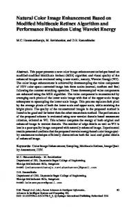
Figure 1: Style enhancement results. (a) Original photo taken by iPhone 3G, (b) enhanced photo that mimics the color and tone style of Canon EOS 5D Mark Π; (c) Original photo, (d) enhanced photo with a style learned from a photographer.

Abstract

ferent photographs. As another example, it is well-known that photographs taken by different digital cameras have varying degrees of tone and color discrepancies. This is because each type of camera has its own built-in radiance and color response curves. We define a tone and color style as a set of explicit or implicit rules or curves governing tonal and color adjustments.

Color and tone adjustments are among the most frequent image enhancement operations. We define a color and tone style as a set of explicit or implicit rules governing color and tone adjustments. Our goal in this paper is to learn implicit color and tone adjustment rules from examples. That is, given a set of examples, each of which is a pair of corresponding images before and after adjustments, we would like to discover the underlying mathematical relationships optimally connecting the color and tone of corresponding pixels in all image pairs. We formally define tone and color adjustment rules as mappings, and propose to approximate complicated spatially varying nonlinear mappings in a piecewise manner. The reason behind this is that a very complicated mapping can still be locally approximated with a low-order polynomial model. Parameters within such low-order models are trained using data extracted from example image pairs. We successfully apply our framework in two scenarios, low-quality photo enhancement by transferring the style of a high-end camera, and photo enhancement using styles learned from photographers and designers.

Manually adjusting the tone and color of a photograph to achieve a desired style is often tedious and labor-intensive. However, if tone and color styles can be formulated mathematically in a digital form, they can be automatically and easily applied to novel input images to make them look more appealing. Unfortunately, the rules governing a tone and color style are most often not explicitly available. For instance, it is typically very hard for a photographer to mathematically summarize the rules he uses to achieve a certain impression; and it also involves much work to calibrate the radiance and color response curves of a camera especially considering the fact that color response curves need to cover the entire visible spectrum. Therefore, our goal in this paper is to learn implicit tone and color adjustment rules from examples. That is, given a number of examples, each of which is a pair of corresponding images before and after adjustments, we would like to discover the underlying mathematical relationships optimally connecting the tone and color of corresponding pixels in all image pairs.

CR Categories: I.4.3 [Image Processing and Computer Vision]: Enhancement; I.4.10 [Image Processing and Computer Vision]: Representation—Statistical

For the following reasons, it is challenging to learn tone and color adjustment rules from examples. First, the relationships we need to identify are buried in noisy data available from example image pairs. We need to rely on machine learning and data mining techniques to discover hidden patterns and relationships. Second, the relationships are likely to be highly nonlinear and spatially varying. This is because camera radiance and color response curves are nonlinear, and the adjustment rules used by photographers most likely vary according to tone and color characteristics of local image regions. Third, there may exist other factors in the relationships in addition to the tone and color of individual pixels. For instance, the amount of adjustment may depend on neighborhood statistics which correlate with the material and texture properties of underlying object surfaces.

Keywords: Image Enhancement, Picture Style, Color Mapping, Gradient Mapping, Tone Optimization

1

Introduction

With the prevalence of digital cameras, there have been increasing research and practical interests in digital image enhancement. Tone and color adjustments are among the most frequent operations. While such adjustments often need to be determined on an individual basis, there exist many scenarios where tonal and color adjustments follow common implicit rules. For example, photographers often carefully tune the temperature and tint of existing colors in a photograph to convey specific impressions. For a specific impression, the types of adjustments are usually consistent across dif-

In this paper, we develop a learning based method to achieve our goal. We formally define tone and color adjustment rules as mappings, and propose to approximate complicated spatially varying nonlinear mappings in a piecewise manner. The reason behind this is that a very complicated mapping can still be locally approximated

∗ This work was done when Baoyuan Wang was an intern at Microsoft Research Asia.

1

To appear in ACM TOG 30(4).

Image Pairs

Leaf Nodes Features along edges

Features away from edges

...

Hierarchical Feature Sub-space Division

Feature Extraction

Image Registration

Train Gradient Mappings

Non-leaf Nodes

Train Binary Classifier

Hierarchical Feature Sub-space Division

A Color Mapping Tree: Ctree

Train Color Mappings Leaf Nodes

A Gradient Mapping Tree: Ttree

...

...

Figure 2: The training stage. Leaf nodes are colored in green while intermediate nodes are colored in yellow.

with a linear or low-order polynomial model. Thus, to tackle the complexity and nonlinearity, we adopt a divide-and-conquer strategy by first dividing a feature space into a number of subspaces and then approximating the tone and color mappings within each subspace with a low-order model. Parameters within such low-order models are trained using data extracted from example image pairs. In theory, as long as the mappings exist, they can be approximated to a high precision if the feature space is subdivided into a sufficient number of subspaces.

input images without learning parametric models for such adjustments. Gradient domain image editing techniques and systems have been presented in [Fattal et al. 2002; Perez et al. 2003]. Fattal et al. introduces an effective method for high dynamic range compression by strategically reducing the magnitude of image gradients. Perez et al. presents a framework for gradient domain image editing by altering and re-integrating the original gradient field. An important difference between these existing techniques and our approach in this paper is that our approach identifies the connections between gradients from photos with two different styles and model such connections as parametric gradient mappings, while the above techniques only perform gradient domain adjustments to individual input images without training parametric models.

More specifically, we have the following contributions in this paper. First, we develop a systematic framework for learning complicated tone and color styles from examples. The original feature space is divided into subspaces using binary classification trees. Every leaf node in a classification tree corresponds to a subspace, where a distinct pair of local color and gradient mappings are trained. Second, we identify effective low-order parametric models for local color and gradient mappings. The local gradient mappings are particularly effective for contrast enhancement. Effective techniques have also been developed for luminance channel optimization and spatially coherent color mapping. Third, we apply this framework in two scenarios. In the first scenario, we learn the picture style of a high-end digital camera and use that style to enhance photographs taken by low-end cameras. In the second scenario, we learn styles of images manually enhanced by photographers, and the learned styles can be successfully applied to novel input photographs as well.

Our work has been inspired by previous work on image enhancement, including automatic methods for exposure correction, contrast enhancement and color correction as well as interactive techniques for tonal and color adjustments.

Much work has been performed on image color transfer [Reinhard et al. 2001; Chang et al. 2005; Piti and Kokaram 2007]. Typically, such a method performs a statistical analysis to impose the color characteristics of a reference image onto another source image. Though much progress has been made, the quality of the results still relies on the compatibility between source and reference images as pixelwise correspondences between them do not exist. Based on techniques in image search, cosegmentation and color transfer, Dale et al. [2009] developed a multi-purpose image enhancement framework that leverages a large database of images. Color transfer results are used as training data for learning local parametric mappings. A significant difference between such color transfer based techniques and our work is that color transfer only transfers colors from one or multiple reference images to the source image and any mappings obtained during this process only work for a specific source image while our work in this paper attempts to train a set of tone and color mappings that are generally applicable to a class of images so that users do not need to choose a reference image for each source image.

Inspired by a model of the lightness and color perception of human vision, Jobson et al. [1997] proposed a multiscale center/surround retinex that achieves simultaneous dynamic range compression, color consistency, and lightness rendition. It is essentially a multiscale framework that simultaneously performs local and global color and contrast adjustments. Bae et al. [2006] performs automatic local and global tonal adjustments to an input image to make its local and global contrasts similar to those of a reference image. Lischinski et al. [2006] introduced an interactive local tone adjustment method based on a sparse set of scribbles. Cohen-Or et al. [2006] performs color adjustment according to harmonization rules. Shapira et al. [2009] proposed an interesting method to edit image appearances interactively using Gaussian mixture models (GMMs). Wang et al. [2010] presents a method for adjusting the color composition of an image to match a predefined color theme. All these techniques directly perform tonal or color adjustments to individual

Siddiqui and Bouman [2008] developed a multi-stage color correction algorithm for enhancing digital images obtained from low quality imaging devices such as cell phone cameras. In this framework, a pixel color is classified into a category using a Gaussian mixture model and local color correction is performed using an affine transform specifically tailored for that category. The parameters in the Gaussian mixture model and affine transforms are learned in an offline training procedure. The differences between our work and [Siddiqui and Bouman 2008] are summarized as follows. First, we perform color correction and contrast enhancement simultaneously in the same framework while [Siddiqui and Bouman 2008] only performs color correction. Second, in our work, color adjustments are performed using quadratic models instead of affine models. Figure 4 demonstrates that quadratic models outperform affine models. Third, more importantly, the image and pixel categories adopted in [Siddiqui and Bouman 2008] are only suitable for imag-

2

Related Work

2

To appear in ACM TOG 30(4). ing devices but not for photographers’ stylistic adjustments while the pixel categories in our method are automatically extracted from training data using hierarchical clustering.

To improve image contrast, we further apply local luminance gradient mappings to luminance gradients along the edges (Section 5.2), leaving other pixel gradients unchanged. This is followed by a tone optimization step (Section 5.3), which relies on both the mapped luminance gradients as well as the luminance channel of the previously mapped colors. The result from tone optimization is a new luminance channel that replaces the luminance channel of the previously mapped colors.

Global image enhancement techniques and pipelines have been presented in [Battiato et al. 2004; Kang et al. 2010]. In [Kang et al. 2010], global parameters for image enhancement are trained using personalized enhancement examples. In contrast, our method trains local parametric models instead of global parameters.

3

4 Learning Color and Gradient Mappings

Overview

In this section, we present our methods for feature space subdivision as well as for constructing the two mapping trees. The CIE L∗ a∗ b∗ color space is used in both mapping trees.

Our example-based framework requires a training stage during which color and tone mappings are learned from example image pairs. Once these mappings have been obtained, they can be applied to new images to enhance a certain color and tone style. These training and application phases are illustrated in Figures 2 and 3, respectively. Note that most of the algorithms in this paper perform in the CIE L∗ a∗ b∗ color space.

4.1

Hierarchical Feature Space Subdivision

Let (pl , ph ) be a pair of corresponding pixels such that pl ∈ Iil and ph ∈ Iih . A feature vector for this pair of pixels is defined by collecting all statistical features computed for pl and ph into a single vector. Since we adopt a piecewise approximation approach, we partition the entire set of feature vectors collected from all training image pairs into a number of subsets using binary hierarchical clustering [Ding and He 2002]. Each leaf node of the resulting binary tree represents one bottom-level feature cluster.

Training Stage To learn a certain style from training examples, we first collect a number of representative training image pairs, l h {Iil , Iih }m i=1 . The two images, Ii and Ii , in each pair should be photographs of the same object or scene. Iih should have the intended color and tone style while Iil does not. They are required to have accurate pixelwise registration between them.

There exist multiple choices to define feature subspaces according to clustering results. One simple scheme would be based on Euclidean distance to cluster centers. It is equivalent to constructing a Voronoi diagram for the cluster centers in the feature space. The Voronoi cell for a cluster center defines the feature subspace corresponding to the cluster. However, a cluster center is only the mean of all feature vectors in the same cluster, and does not take into account the boundary shape and spatial distribution of individual clusters.

Our basic idea is to learn hidden relationships between the color and tone of registered pixels. To effectively learn a style transformation, we propose to train color mappings using corresponding pixels in the image pairs. In general, such mappings are highly nonlinear and spatially varying. Finding a single closed-form parametric model for such mappings is an elusive task. We decide to represent these mappings in a piecewise manner.

We take an alternative approach, which, at every intermediate node of the binary tree, obtains a partition surface that optimally separates feature vectors in the left subtree from those in the right subtree. We use the decision surface of a binary classifier to serve this purpose. In our current implementation, we use kernel support vector machines (SVMs) [Vapnik 1995] and the RBF kernel. When training an SVM, we use feature vectors in one subtree as the positive training examples and feature vectors in the other subtree as the negative training examples. Under this scheme, to locate the optimal subspace for a feature vector, one only needs to test it against O(log(n)) classifiers on a path from the root to a leaf. Here n is the number of leaf nodes.

We extract local statistical features from neighborhoods centered at every pixel in both images of every training pair. The features may include the average and standard deviation of colors within a neighborhood as well as gradient information. Let F be a multidimensional feature space where feature vectors extracted from training images reside. We build a binary feature space partition tree that divides F into n subspaces (leaf nodes), F1 , F2 , . . . , Fn , so that F = F1 ∪ F2 ∪ F3 ∪ . . . ∪ Fn . All feature vectors contained in each leaf node define one feature subspace, and we train a local color mapping specifically tailored for that feature subspace. All subspace color mappings constitute our final piecewise approximation of the overall nonlinear color mapping.

Table 1: Comparison of root mean squared errors (RMSE) between a classifier based method and a cluster center based method on four groups of testing data. RMSEs were measured for the three channels of the CIEL∗ a∗ b∗ color space separately.

Since luminance gradients along edges can significantly affect the overall image contrast, we further build a second binary feature space partition tree related to luminance gradients, and train local mappings for luminance gradients along edges. The output of this training stage consists of two binary space partition trees: one for color mapping, and the other for luminance gradient mapping (Figure 2).

Group # 1 Group # 2 Group # 3 Group # 4

Style Enhancement Once having obtained the aforementioned two trees, we can apply the local mappings in these trees to adjust the color and contrast of a given image to enhance the intended style. We first segment the input image into multiple soft segments, and then apply the trained local color mappings to adjust the colors of the soft segments in a spatially coherent manner. This color mapping step will be elaborated in Section 5.1.

Classifiers 0.076, 0.049, 0.033 0.088, 0.046, 0.078 0.073, 0.042, 0.077 0.091, 0.043, 0.044

Cluster Centers 0.154, 0.241, 0.093 0.130, 0.075, 0.086 0.118, 0.074, 0.112 0.144, 0.076, 0.079

Our experiments show that using classifiers to locate the optimal subspace for a new incoming feature vector is more accurate than the simple scheme based on Euclidean distance to cluster centers. This is illustrated in Table 1, where for each group of testing data, these two different methods locate the optimal subspaces on their own, and then apply the color mappings associated with the found

3

To appear in ACM TOG 30(4).

Edge Pixels

Input Image

Locate Subspaces In Ttree

Gradient Mappings

Tone Optimization

Soft Segmentation

Output Image All Pixels

Locate Subspaces In Ctree

Color Soft Blending

Color Mappings

Figure 3: Image enhancement pipeline.

subspaces. We confirmed that the RMSE of the color mapping results for the classifier based method are smaller than that for the cluster center based method. We measured the RMSEs for all three channels of the CIEL∗ a∗ b∗ color space. This result demonstrates that classifier based subspace search can achieve more accurate results.

4.2

Learning Local Color Mappings

-2

Colors associated with pixels whose feature vectors belong to a feature subspace are used for training a local color mapping for that feature subspace. Since we approximate the global color mapping in a piecewise manner by dividing the feature space into a number of subspaces, we expect each local color mapping to be accurately represented by a low-order parametric model.

(1)

where (A, b) define an affine transformation between Qj and chj , A is a 3x3 matrix for a linear basis and a 3x9 matrix for a secondorder polynomial basis, and b is always a 3-vector. Given a sufficient number of corresponding pixels associated with a feature subspace, A and b can be easily solved by minimizing the following least-squares objective function.

A,b

N 

AQj + b − chj 2 ,

2 1.5

1

1

0.5

0.5

0 -0.5 0

2

-2

0 -1 -0.5 0

-1

-1

-1.5

-1.5

-2

-2

1

2

Analysis (CCA) [Hardoon et al. 2004], which is a standard method for multivariate correlation analysis. CCA is capable of identifying pairs of basis vectors for two sets of observations such that the correlation between the projections of the original observations onto these basis vectors are mutually maximized. Our experiments show that the quadratic model achieves overall better correlation results. Figure 5 compares the correlation results between the linear model and quadratic model, respectively. Obviously, a better correlation is achieved when Qj is set up as a second-order polynomial basis, which indicates that the mapping between clj and chj is slightly nonlinear. In fact, higher-order polynomial models should have even better correlation results. Nonetheless, higher-order models have a larger degree of freedom, therefore, are more likely to suffer from overfitting.

We define a local color mapping as follows.

arg min

2 1.5

Figure 5: Comparison of correlation results for the linear and quadratic color mapping models.

Let (plj , phj ) be a pair of corresponding pixels from the training images. Let clj = (Llj , alj , blj ) be the CIE L∗ a∗ b∗ color vector at plj and chj = (Lhj , ahj , bhj ) be the CIE L∗ a∗ b∗ color vector at phj . Let Qj be a polynomial basis vector defined for clj . alj blj )T for a linear basis and For example, Qj = (Llj l2 l2 h2 l l l l Qj = (Li ai bi Li ai Li bi ali bli Lli ali bli )T for a second-order polynomial basis.

chj = AQj + b,

Quadratic Model ( correlation = 0.88 )

Linear Model ( correlation = 0.59 )

4.3

Learning Mappings for luminance Gradients

Since luminance gradients along edges can significantly affect the overall image contrast which in turn is an important factor of an image tone style, we further build a second binary feature space partition tree related to luminance gradients, and train a local luminance gradient mapping for every leaf node of the tree.

(2)

j=1

where N is the number of corresponding pixels, each of which defines three additional constraints since a color vector has three channels.

Recall (plj , phj ) is a pair of corresponding pixels from the training images, Llj and Lhj are their luminance channels in the CIE L∗ a∗ b∗ color space. Since image contrast is typically adjusted using the gamma correction, we model a local mapping between corresponding luminance values using the following power law,

Previous work on image color transfer and color correction often adopts the linear basis for color mapping. Our experiments show that the linear basis can produce reasonably good results in most cases, however, the second-order polynomial basis can model color mappings more accurately especially when there exist subtle color distortions. This has been demonstrated in Figure 4, where the overall visual difference between the enhanced result and the reference image is smaller when the quadratic model is used.

γ

Lhj = Llj .

(3)

Taking the logarithm of the gradient of both sides, we obtain

In addition to visual results, we have also explored the underlying correlation between Qj and chj using Canonical Correlation

ln

4

∇Lhj  = ln γ + (γ − 1) ln Llj . ∇Llj 

(4)

To appear in ACM TOG 30(4).

Figure 4: (A) is an original photo taken by iPhone 3G while (D) is the reference photo taken by Canon 5D Mark Π. (B) is the result from an affine color mapping while (C) is the result from a quadratic color mapping. Between (B) and (C), (C) is overall visually closer to (D).

We can easily verify that the right-hand side of (4) is just a linear transformation of the log-luminance of the pixel plj . Hence, instead of estimating γ directly, we generalize the relationship in (4) to a generic linear mapping, and solve the parameters in this linear mapping by minimizing the following least-squares objective function,  2 N  ∇Lhj  l α + β ln Lj − ln , (5) arg min α,β ∇Llj  j=1

first select the pixels whose probability for that segment is larger than 0.5. Then we build a subspace voting histogram H, whose bins correspond to the leaves of the color mapping tree. For each of the selected pixels, locate the subspace its feature vector belongs to and increment the counter in the corresponding histogram bin. For each soft segment, we choose the three most frequently visited subspaces and their associated local color mappings. Suppose the three chosen mappings for the t-th segment are (Atj , btj ),j = 1, 2, 3, and the values of the corresponding normalized histogram bin counters are λtj , j = 1, 2, 3. We apply these three chosen mappings to all pixels in the t-th segment as follows,

where α and β are the parameters in the linear mapping. Once the parameters have been solved, the luminance gradient mapping is formulated as ∇Lhj = ∇Llj exp(α + β ln Llj ).

˜ti = c

(6)

3 

λtj (Atj Qi + btj ),

(7)

j=1

5

Color and Tone Style Enhancement

where Qi is the second order polynomial basis vector for the original color of the input image at pixel i. After this within-segment blending, the final color of each pixel is further blended according to soft segmentation probabilities. That is, the final color of pixel i is computed as K  ˜ti . ˜ Pit c (8) ci =

In this section, let us discuss how to make use of the trained local color and luminance gradient mappings to perform image color and tone style enhancement.

5.1

Spatially Coherent Color and Tone Mapping

t=1

Given the trained binary feature space partition tree and the local color mappings at the leaf nodes, for every pixel in a new input image, we may first extract its feature vector, then simply go through the binary tree to locate the subspace the feature vector belongs to, and finally apply the local color mapping associated with that subspace to the color channels of the pixel to obtain a new color. However, this straightforward process could give rise to noisy color mapping results because subspace search for neighboring pixels is carried out independently, and two adjacent pixels may end up within two different subspaces with different color mappings.

5.2

Luminance Gradient Mapping

Since luminance gradients along edges significantly affect the overall image contrast, in addition to color and tone adjustments based on local color mappings, we further apply local mappings of luminance gradients to enhance the contrast of an input image. As in the previous subsection, given the feature vector of an edge pixel, we search for the subspace this feature vector belongs to in the binary feature space partition tree for luminance gradients, and apply the local luminance gradient mapping associated with that subspace to obtain a new luminance gradient at the edge pixel. The computation of the new luminance gradient follows (6). Unlike color mapping, luminance gradient mappings are applied to individual edge pixels independently without considering spatial coherence.

We introduce a segmentation-based mapping technique that can achieve spatially coherent mapping results. We first divide an input image into multiple soft segments, each of which associates one probability value with every pixel. All probability values at a pixel sum up to one. To remove potential ambiguity, we further require that the largest probability value at every pixel be larger than 0.5. The soft segment associated with this largest value is the dominant segment at the pixel. Our soft segmentation process is similar to the one in [Wang et al. 2010] except that we rely on the instant edit propagation method in [Li et al. 2010] to extract soft segments.

In our experiments, we use the Canny edge detector to find edge pixels. A Canny edge is only one-pixel wide. Therefore there exist jaggies along an edge. Enhancing the gradients along Canny edges can only make edge artifacts stand out, resulting in unnatural enhancement results. In practice, we sample additional pixels with a large gradient in a 5x5 local neighborhood of each edge pixel, and apply luminance gradient mappings to these sampled pixels as well. The luminance gradients at the rest of the pixels are left unchanged.

Suppose there are K (usually from 5 to 12) soft segments. Let Pit be the probability value for the t−th segment at the i-th pixel, where t = 1, 2, . . . , K, i = 1, 2, . . . , N . For each segment, we

5

To appear in ACM TOG 30(4).

Figure 6: (A) is an original photo taken by iPhone 3G. (E) is the reference photo taken by Canon 5D Mark Π. (B) is obtained with both color mapping and tone optimization, but a feature vector only consists of three color channels. (C) is obtained directly from color mapping as in (8) without additional tone optimization. (D) is our final result with color and gradient mappings, tone optimization, and a feature vector includes additional neighborhood statistics other than color channels.

5.3

Tone Optimization

enhancement by transferring the style of a high-end camera, ii) enhancing digital photos using styles learned from photographers and designers.

Color mapping as formulated in (7) and (8) computes a newly mapped luminance value for every pixel since luminance is one of the three channels in the CIE L∗ a∗ b∗ color space. Luminance gradient mapping as formulated in (6) computes a newly mapped luminance gradient for a subset of pixels including the edge pixels. At the end, we would like to perform tone optimization to produce a new luminance channel that is maximally consistent with both of these mapped luminance values and luminance gradients.

6.1

Nowadays, more and more people prefer to take pictures of their daily life at any time, anywhere using their cell phone cameras. This is because people tend to bring their cell phones every day but not a digital camera due to the convenience. Although cell phone cameras have gained incredible development over the past years, for example, the most popular iPhone 4 camera can take pictures with nearly 5 Mega pixels, the image quality is still not comparable to Digital Single Lens Reflex (DSLR) cameras. Typical defects, that exist in photos taken by cell phone cameras, include color infidelity, poor contrast, noise, incorrect exposure and so on even though the resolution is already very high.

˜ i be the mapped luminance value at pixel i, and gi be the lumiLet L nance gradient vector at pixel i. At pixels that underwent luminance gradient mapping, gi represents the newly mapped luminance gradient; otherwise, it represents the original luminance gradient in the input image. The aforementioned tone optimization can be formulated as the following least-squares minimization,  ˆ i − gi 2 + (L ˆi − L ˜ i )2 ), (wi ∇L (9) arg min ˆ L

In this paper, we focus on increasing color fidelity and improving contrast for photos taken by a low-end cell phone camera because color infidelity and poor contrast cannot be easily corrected and enhanced by simple adjustments in a global manner even using commercial software such as Adobe Photoshop. We try to achieve these goals by transferring and mimicking the color and tone style of a high-end camera. This is because the high-end camera has better contrast and color fidelity. By using photos taken by the high-end camera as the ground truth, our results can be easily validated by comparing the enhanced photos against the ground truth. It is wellknown that standards on photo quality are highly personalized. Our approach, to a certain extent, makes photo enhancement become a more objective task.

i

ˆ is the unknown new luminance channel that needs to be where L solved, and wi is a spatially varying weighting coefficient. In practice, the value of wi at edge pixels is set to be one order of magnitude larger than its value at the rest of the pixels to emphasize the consistency between the gradient of the solved lumiˆi nance channel and the mapped gradient in (6). If we replace ∇L with finite differences, (9) becomes a linear least-squares problem and its normal equation is a sparse linear system that can be efficiently solved using an existing sparse linear solver, such as Taucs [Toledo et al. 2003]. Note that if the spatially varying weight wi is replaced with a constant weight, the normal equation of (9) becomes equivalent to the screened Poisson equation [Bhat et al. 2008].

Data Collection We chose two recently popular cell phones iPhone 3G and Android Nexus One as the low-end cameras, and Canon EOS 5D Mark Π as the high-end DSLR camera, which can take high quality photos thanks to its high-end CCD sensors as well as the embedded image processing software. Our goal is to learn the color and gradient mapping models between a low-end camera and the high-end DSLR camera. Photos were taken for both indoor and outdoor scenes with diverse colors and under different illumination conditions. For each scene, we first took a photo using a low-end camera, then took a corresponding high-quality photo from the same viewpoint. By manually adjusting the focal length of the high-end camera, we made corresponding photos overlap as much as possible.

Finally, we replace the luminance channel estimated in (8) with the new luminance channel obtained from (9) to complete our color and tone style enhancement. Figure 6(D)&(C) show a pair of results obtained with and without tone optimization. Although compared with the input (A), (C) is visually closer to the reference photo (E), the bottom part of (C) still suffers from poor contrast. Because of luminance gradient mapping and tone optimization, (D) is visually closest to (E) in both color and contrast.

6

Photo Enhancement by Style Transfer

Applications and Results

There exists much redundancy among the original photos. Hence, we manually chose a subset of representative photos as our experimental data. More specifically, we chose 110 pairs for iPhone 3G

In this section, we apply our color and tone style enhancement approach in two application scenarios: i) low-quality digital photo

6

To appear in ACM TOG 30(4). #of subspaces VS average correlation 0.9 0.85 0.8 0.75 0.7 0.65 0.6 0.55 0.5 0.45 0

100

200

300

400

500

Figure 8: Relationship between the number of subspaces and the average correlation for all subspaces. Correlation analysis is performed between the input and output of the local mappings. We adopt Canonical Correlation Analysis (CCA) [Hardoon et al. 2004] to perform this task.

Figure 7: A subset of training image pairs. The top four were taken by iPhone 3G while the bottom four by Canon 5D Mark Π.

versus Canon and 72 pairs for Android phone versus Canon. Each of these datasets was further randomly divided into two equal subsets. We took the first subset as training data and the second one as testing (validation) data. Figure 7 shows four pairs of training images.

Color moments are affine invariant and have a reasonably strong discriminative power over local color variation patterns. Image gradients (both orientation and magnitude) also have a strong discriminative power over local shapes and patterns. The motivation behind color correlation matrices is that, for 1-CCD color cameras, color filters on the pixel array of an image sensor typically follow the Bayer arrangement, which only places one of the three possible color filters over each pixel. Interpolation must be performed to reconstruct all three color channels for a pixel using color channels available from its neighboring pixels. Therefore, nearby pixel colors of such cameras are inherently correlated. Furthermore, such interpolation causes color distortion itself because different color channels have different interpolation masks.

Luminance Normalization and Image Registration Because photos taken by two different cameras are not registered by default, we need to perform pixel-level registration between every pair of images used in the training stage. Before registration, we perform luminance normalization, which improves luminance consistency among photos and increases registration accuracy. We convert all photos from the RGB color space to the CIE L∗ a∗ b∗ color space. This conversion involves an inverse gamma correction, which removes most of the nonlinearity caused by the camera’s radiance response curve. We further normalize the average luminance of every photo to 0.65. Most digital photos are taken in the auto-exposure mode and different cameras have different exposure control mechanisms. By normalizing the average luminance, we eliminate inconsistent luminance levels caused by automatic exposure and make photos taken by different cameras comparable. For a new testing ¯ and multiply the lumiphoto, we compute its average luminance L ¯ to adjust its average luminance to nance of every pixel by 0.65/L 0.65. After enhancement, we adjust back by multiplying the lumi¯ nance of every pixel in the enhanced photo by L/0.65.

For the high-end camera, we only extract the luminance gradient as well as the pixel color as the per-pixel features. These extracted features are used in feature clustering, feature space partitioning, and feature vector classification. The comparison shown in Figure 6(B)&(D) demonstrates that it is necessary to include additional neighborhood statistics in a feature vector. Figure 6(B) was obtained by running our complete enhancement pipeline except replacing the aforementioned 27-dimensional feature space with the three-dimensional CIE L∗ a∗ b∗ color space. From this result, we can infer that local color and gradient mappings are not only correlated with individual pixel colors, but also correlated with neighborhood statistics.

To reduce the computation overhead, we scale the two photos in each pair to the same resolution (512x512 in our experiments) by down-sampling and cropping. Then we use a revised version of the image matching algorithm in [Shinagawa and Kunii 1998] to perform registration between them. Since automatic image registration is error prone, we further made the registration process iterative and interactive to achieve accurate registration results. Once an automatic result is generated, the user can interactively lasso well-matched regions, and sample pixels within the regions. The sampled pixels are set as additional hard correspondences in the next iteration of optimization, and such hard constraints will propagate to coarser levels of the multiresolution pyramid to guide the matching process there.

Training Based on the above setup, we have trained enhancement models for both iPhone versus Canon and Android versus Canon. For each type of cell phone, we trained two distinct enhancement models for indoor and outdoor scenes due to very different spectra of the light sources in indoor and outdoor scenes. In our experiments, we typically divide the feature space for gradient mapping into 200 subspaces and the feature space for color mapping into 300 subspaces. We may overfit with an overly large number of subspaces or underfit with an insufficient number of subspaces given a fixed number of training examples. To achieve both good approximation and generalization capabilities, we determine the number of subspaces by checking the average correlation between the input and output of the local mappings for all the subspaces using canonical correlation analysis again. Such a correlation analysis indicates that the average correlation increases with the number of subspaces when this number is relatively small but tends to stabilize when this number exceeds a threshold. This is shown in Figure 8, which indicates the number of subspaces should be chosen between 200 and 300.

Feature Selection For the photos taken by iPhone and Android phones, we extract the following features at every pixel: the first three moments of the three channels of the CIE L∗ a∗ b∗ color space in a local window (7x7) centered at the pixel; the gradient vectors of the three color channels at the pixel; the color correlation matrix of the three color channels in the same window for displacement vectors defined by half of the eight pixels in a 3x3 neighborhood. This results in a 27-dimensional feature vector.

7

To appear in ACM TOG 30(4).

(A)

(C)

(B)

(D)

Figure 10: (A) Original photos taken by Panasonic DMC-LX3GK. (B) Calibrated photos by Macbeth color checker. (C) Our results. (D) Reference photos taken by Canon 5D Mark Π. Our results are closer to the reference photos. Table 2: Comparison of average and standard deviation (SD) of RMSEs of the RGB channels between original and enhanced lowquality photos, and comparison of average and standard deviation of the root mean squared L2 distances in the 3D CIELAB color space, denoted as D, between original and enhanced low-quality photos.

Average SD

Before Enhancement (R G B) D

After Enhancement (R G B) D

(0.108, 0.112, 0.183) 0.076 (0.042, 0.048, 0.056) 0.015

(0.081, 0.074, 0.075) 0.037 (0.039, 0.039, 0.029) 0.014

L2 distances among all testing images. The results are summarized in Table 2, where we confirm that both types of errors have been significantly reduced after the application of our enhancement. Figure 9: Left: Original photos (the top one was taken by Android Nexus One while the bottom one was taken by iPhone 3G). Middle: Our enhanced results. Right: Reference photos taken by Canon.

Figure 9 shows visual results for two testing photos, which are among the most challenging examples in our testing data. Figures 1, 11 and the supplementary materials show additional visual results. The weight, wi , in (9) is the only adjustable parameter in our algorithm. In all our experiments, its value is set to 10 at edge pixels and sampled pixels near the edges, and 1 at the rest of the pixels. The major cost of our algorithm lies in locating the optimal subspaces. This is because every pixel in a testing photo needs to go through multiple classifications in the binary feature space partition trees before reaching any local mappings associated with the leaf nodes. For a 512X512 input photo, it takes 3 minutes to perform the overall gradient and color mappings, and 2 seconds to perform the tone optimization by solving the sparse linear system. Our timings were obtained on an Intel Xeon 2.33GHz processor with 2GB RAM. This process can be significantly accelerated by multicore processors or modern GPUs since pixelwise classification and mapping are independently performed at every pixel and can thus be easily parallelized.

Since we have partitioned the original datasets into two halves, one for training and the other for testing, we use the testing data to validate our proposed method. Both visual and quantitative testing results demonstrate that our method can successfully model underlying color and tone relationships between two types of cameras.

Testing and Validation

To evaluate the numerical accuracy of our learned mappings, we first perform pixel-level registration between photos in every testing image pair using our revised version of the image matching algorithm in [Shinagawa and Kunii 1998]. Then we apply our method to enhance the low-quality photo in every testing image pair while using the high-quality photo in the same pair as a reference. Afterwards, we compare both the original and enhanced low-quality photos with the reference through matching pixels obtained during registration, and calculate the root mean squared error (RMSE) for both the original and enhanced low-quality photos. We also calculate the root mean squared L2 distances in the CIELAB color space for both the original and enhanced low-quality photos. Finally, we compute the average and standard deviation of such RMSEs and

Comparison with Color Checker Calibration The Macbeth color checker is a well-known color chart for color calibration. It has a 4x6 array of standardized color samples with ground-truth color coordinates. When the Macbeth color checker is used for cal-

8

To appear in ACM TOG 30(4).

Figure 11: Photo enhancement results using the style of a high-end camera. Top: Original photos of indoor and outdoor scenes (the leftmost one was taken by Android Nexus One, while the other three were taken by iPhone 3G). Middle: Enhanced results. Bottom: Reference photos taken by Canon.

ibrating the color of a camera, one needs to first take a photo of the color checker under an intended illumination condition, and a calibrating software, such as Adobe Lightroom, compares the color coordinates of the color samples in the photo against their groundtruth color coordinates to work out a calibration profile, which is then applied to any subsequent photos taken by the same camera under a similar illumination condition.

reference photo taken by the high-end camera.

6.2

Learning Color and Tone Styles from Photographers

Photographers often carefully tune the temperature and tint of existing colors in a photograph to evoke certain impressions or mood. For a specific impression, the type of adjustments are usually consistent across different photographs. Nevertheless, the tuning process is tedious and time-consuming. It is much desired to automate this process. However, it is hard to explicitly summarize the rules a photographer uses to achieve a certain impression. We attempt to learn such implicit photo enhancement rules from examples. That is, if we have a set of images manually enhanced with a certain impression by photographers and use the original and enhanced images as training image pairs, we can learn the implicit color and tone style adjustment rules used for achieving the enhanced results. Once the styling rules have been learned in the form of color and gradient mappings, they can be applied to novel input images to achieve a desired impression automatically.

Although the Macbeth color checker is a useful tool for generic color calibration, it would not be a good fit in the context of learning the color style of a camera for the following reasons. First, the twenty four color samples on a color checker only form a very sparse sampling of an entire 3D color space. Any color reasonably far away from all the color samples may not be calibrated very accurately. Thus, a color checker cannot provide very accurate calibration for the entire color space. Second, the color checker can only recover the true color coordinates of its color samples but not the color coordinates that would be produced by a specific camera. This is because even a high-end camera may produce color coordinates that are slightly different from the ground truth. We performed a comparison between our color style enhancement and color calibration with a color checker using Panasonic DMCLX3GK, a relatively low-end digital camera that can output images in the ”RAW” format. This is because color calibrating software requires the ”RAW” format while cell phone cameras cannot output images in this format. Being able to handle images not in the ”RAW” format is thus an additional advantage of our technique. The comparison results are shown in Figure 10, where we can clearly verify that the color checker can only obtain accurate results on a subset of colors while our results are much closer to the

Training Data To prepare our training data, we started with a collection of photographs of both natural and urban scenes, and performed soft image segmentation on each of them. The reason for image segmentation is that distinct color and tone adjustments can be applied to different segments to achieve sophisticated editing effects. Meanwhile, we invited several photographers to perform local color and tone adjustments to these segmented images using our custom-developed user interface. We asked each of the pho-

9

To appear in ACM TOG 30(4). tographers to conceive a color and tone style and try his/her best to enhance the conceived style in a subset of the segmented images. Since different photographers most likely had different styles in mind, we did not mix images enhanced by different photographers together. We define one training dataset for our style learning as a subset of original photographs plus their corresponding images enhanced by the same photographer. In each training dataset, we have collected around 20 pairs of training images. Figure 12 shows training images from two different styles. Since each pair of training images is by default registered, we do not need to run image registration in this application. We train a distinct set of color and gradient mappings for every style. The number of subspaces for gradient and color mappings are 100 and 150, respectively.

Figure 14: Comparison between our method and color transfer by [Piti and Kokaram 2007]. Our enhanced result is based on the first style in Figure 13.

Figure 12: A subset of training examples for two different styles. Top: Original photos. Bottom: Photos enhanced by two photographers (the left two belong to the first style, and the right two belong to the second style).

ent colors and intensities, the total number of images in a training dataset does not need to be very large. Our color and gradient mappings can already produce reasonably good results given a dozen or so representative training image pairs. Another issue is that we require pixel-level image registration within every training image pair, especially when the two images in a pair are taken by different cameras. Such a level of precision is not easy to achieve with existing image registration algorithms. As a result, we had to rely on user-provided hard constraints to improve automatic registration results. Providing such constraints requires a certain amount of manual work.

Results Once the styling rules have been learnt, we can apply them to novel input photos to enhance the desired style. Experiments show our method can produce vivid results with the same style as manually tuned by the photographers. Figure 13 shows photos enhanced with two different styles using our method. Comparisons between our enhanced results and manually tuned results by photographers can be found in the supplemental materials.

We have also measured the performance. For a 512x512 photo, it usually takes 2 mins to perform both the gradient and color mappings since the mapping trees have a smaller size in this scenario.

Acknowledgements We would like to thank Sing Bing Kang, Wenping Zhao, Hao Li for helpful discussions and the anonymous reviewers for their valuable comments. This work was partially supported by National Science Foundation (IIS 09-14631).

Color transfer [Piti and Kokaram 2007] is the most relevant work in this application. To perform color transfer to an input image, one must provide a suitable reference image with the desired style. In addition, the quality of the results is highly dependent on the consistency of color statistics between the two images. Users may need to perform a large number of trials before obtaining a reasonable result. Figure 14 shows a comparison of enhanced photos obtained from both our method and color transfer.

7

References BAE , S., PARIS , S., AND D URAND , F. 2006. Two-scale tone management for photographic look. In SIGGRAPH ’06: ACM SIGGRAPH 2006 Papers, ACM, New York, NY, USA, 637–645.

Conclusions

BATTIATO , S., B OSCO , A., C ASTORINA , A., AND M ESSINA , G. 2004. Automatic image enhancement by content dependent exposure correction. EURASIP Journal on Applied Signal Processing 12.

In this paper, we have developed a method for learning color and tone styles from examples. This method is capable of discovering underlying mathematical relationships in color and tone between corresponding image pairs. We have successfully applied our framework in two scenarios, low-quality photo enhancement by transferring the style of a high-end camera, and photo enhancement using styles learned from photographers and designers.

B HAT, P., C URLESS , B., C OHEN , M., AND Z ITNICK , L. 2008. Fourier analysis of the 2d screened poisson equation for gradient domain problems. In European Conference on Computer Vision (ECCV).

Limitations. Like most other data-driven techniques, our proposed method requires a training stage where data-driven models are optimized. The performance of the trained data-driven models relies on the quality and quantity of the training data. Fortunately, this is not a serious problem with images. As a typical image already has at least hundreds of thousands of pixels with differ-

C HANG , Y., S AITO , S., U CHIKAWA , K., AND NAKAJIMA , M. 2005. Example-based color stylization of images. ACM Trans. Appl. Percept. 2, 3, 322–345. C OHEN -O R , D., S ORKINE , O., G AL , R., L EYVAND , T., AND X U , Y.-Q. 2006. Color harmonization. In SIGGRAPH ’06:

10

To appear in ACM TOG 30(4).

Figure 13: Photo enhancement results using two styles learned from photographers. Top: Original photos. Bottom: Enhanced results (the left two belong to the first style, and the rightmost one belongs to the second style).

P ITI , F., AND KOKARAM , A. 2007. The linear mongekantorovitch linear colour mapping for example-based colour transfer. Visual Media Production, 4th European Conference on Visual Media Production, London, UK, 1–9.

ACM SIGGRAPH 2006 Papers, ACM, New York, NY, USA, 624–630. DALE , K., J OHNSON , M., S UNKAVALLI , K., M ATUSIK , W., AND P FISTER , H. 2009. Image restoration using online photo collections. In International Conference on Computer Vision (ICCV).

R EINHARD , E., A SHIKHMIN , M., G OOCH , B., AND S HIRLEY, P. 2001. Color transfer between images. IEEE Comput. Graph. Appl. 21, 5, 34–41.

D ING , C., AND H E , X. 2002. Cluster merging and splitting in hierarchical clustering algorithms. In Proceedings of the 2002 IEEE International Conference on Data Mining, IEEE Computer Society, Washington, DC, USA, ICDM ’02.

S HAPIRA , L., S HAMIR , A., AND C OHEN -O R , D. 2009. Image appearance exploration by model-based navigation. Comput. Graph. Forum 28, 2, 629–638.

FATTAL , R., L ISCHINSKI , D., AND W ERMAN , M. 2002. Gradient domain high dynamic range compression. ACM Trans. on Graphics 21, 3, 249–256.

S HINAGAWA , Y., AND K UNII , T. L. 1998. Unconstrained automatic image matching using multiresolutional critical-point filters. IEEE Transactions on Pattern Analysis and Machine Intelligence 20, 994–1010.

H ARDOON , D. R., S ZEDMAK , S. R., AND S HAWE - TAYLOR , J. R. 2004. Canonical correlation analysis: An overview with application to learning methods. Neural Comput. 16 (December), 2639– 2664.

S IDDIQUI , H., AND B OUMAN , C. 2008. Hierarchical color correction for camera cell phone images. IEEE Transactions on Image Processing 17, 11, 2138–2155. T OLEDO , S., ROTKIN , V., AND C HEN , D. 2003. Taucs: A library of sparse linear solvers. version 2.2. Tech. rep., Tel-Aviv University.

J OBSON , D., R AHMAN , Z., AND W OODELL , G. 1997. A multiscale retinex for bridging the gap between color images and the human observation of scenes. IEEE Transactions on Image Processing 6, 7, 965–976.

VAPNIK , V. 1995. The Nature of Statistical Learning Theory. Springer, New York.

K ANG , S., K APOOR , A., AND L ISCHINSKI , D. 2010. Personalization of image enhancement. In IEEE Conference on Computer Vision and Pattern Recognition (CVPR).

WANG , B., Y U , Y., W ONG , T.-T., C HEN , C., AND X U , Y.-Q. 2010. Data-driven image color theme enhancement. ACM Trans. Graph. 29, 5.

L I , Y., J U , T., AND H U , S.-M. 2010. Instant propagation of sparse edits on images and videos. Computer Graphics Forum 29, 2049–2054. L ISCHINSKI , D., FARBMAN , Z., U YTTENDAELE , M., AND S ZELISKI , R. 2006. Interactive local adjustment of tonal values. ACM Trans. Graph. 25, 3, 646–653. P EREZ , P., G ANGNET, M., AND B LAKE , A. 2003. Poisson image editing. ACM Trans. on Graphics 22, 3, 313–318.

11