WINPEC Working Paper Series No.E1610 May 2017
Expected Utility Theory with Probability Grids and Preferential Incomparabilities
Mamoru Kaneko
Waseda INstitute of Political EConomy Waseda University Tokyo,Japan
Expected Utility Theory with Probability Grids and Preferential Incomparabilities∗ Mamoru Kaneko†, May 31, 2017
Abstract We reformulate expected utility theory by separating the measurement of utility from pure alternatives and its extension to lotteries involving risks. At the same time, we introduce cognitive bounds on the depths of permissible probability values; for example, probabilities have only decimal (or binary) fractions of finite depths that are not greater than a given bound. We allow the preference relation in question to be incomplete. When no depth restrictions are given, the axioms determine uniquely a complete preference relation, which can be considered classical expected utility theory. When a finite cognitive bound is given, the axioms allow multiple preference relations including incomparabilities on some lotteries. We give a complete characterization of preferential incomparabilties, and a representation theorem in terms of a 2-dimensional vector-valued utility function. We exemplify the Allais paradox within our theory, and argue that the prediction of our theory is well compatible with the experimental results reported by Kahneman-Tversky when we adopt a very shallow cognitive bound. JEL Classification Numbers: C72, C79, C91 Key words: Expected Utility, Measurement of Utility, Probability Grids, Cognitive Bounds, Preferential Incomparabilities
1
Introduction
Although expected utility (EU) theory plays an important role in economics and game theory, various paradoxes have been reported since Allais [2]. To study such paradoxes, here we restrict available probabilities in EU theory to decimal (`-ary, in general) fractions up to a cognitive k bound ρ; if ρ is a finite natural number k, it is given as Πρ = Πk = { 100k , 101k , ..., 10 }; and if 10k Π . We allow a preference relation to be incomplete. The limit ρ = ∞, it is given as Πρ = ∪∞ k=0 k case with ρ = ∞ can be considered classical EU theory in the sense of von Neumann-Morgenstern [22] (cf., Herstein-Milnor [10] and Hammond [7] for later developments). Our theory indicates where the Allais paradox emerges and shows how it may be avoided. k } may be interpreted as a partition of For a finite k, the set of grids Πk = { 100k , 101k , ..., 10 10k ∗
The author thanks P. Wakker, J. J. Kline, M. Lewandowski, L. Tang, A. Dominiak, and S. Shiba for helpful comments on earlier versions of this paper. The author is supported by Grant-in-Aids for Scientific Research No. 26245026, Ministry of Education, Science and Culture. † Waseda University, Tokyo, Japan (
[email protected])
1
Measurement Axioms B1 to B3 Base Facet F
bound 2
Preference relations Y (pure) Axioms B0: Transitivity
lotteries lotteries . . . of depth 1 of depth 2
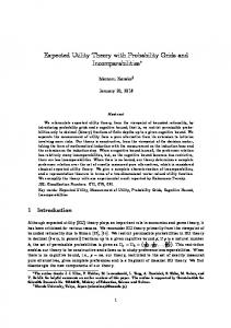
Extension Axiom B4
Figure 1: From Simple to Complex the continuum [0, 1] so that the grids in Πk represent the components in the partition. We take, however, the opposite view that a set of grids is, cognitively and theoretically, more primitive than [0, 1]. Our development goes from shallower to deeper cases; the decision maker thinks about his evaluation with a small k to larger k’s up to a given bound ρ. Even when ρ = ∞, Πρ = ∪∞ k=0 Πk does not reach the continuum [0, 1] and it is still a subset of the set of rational numbers. We are particularly interested in cases of finite cognitive bounds, and the limit case is the reference point. In this sense, our theory deals with “bounded rationality” due to Simon [19], [20]; Simon [20] criticized EU theory as a description of “super rationality.” The limit case in our theory is interpreted as corresponding to Simon’s “super rationality”. A hint for our development is found in von Neumann-Morgenstern [22]. They divided the motivating argument into (i) measurement of utility in terms of probability; and (ii ) extension to lotteries involving risks such as plans for future events. This separation, however, is not reflected in their mathematical development. We separate and formulate these steps as mathematical induction, that is, from simple to more complex cases. In particular, we restrict Step (i) to the measurement of utility from a pure (no risk) alternative in terms of two benchmarks and available probabilities. Step (ii ) extends this measurement to lotteries with probabilities of larger depths. As in Figure 1, these steps are described by Axioms B0 to B4. The lotteries with probability grids and a sequence of preference relations h%k iρk=0 prepare the language of our theory; ρ = 2 in Figure 1. These axioms describe the meaning of benchmarks, how the decision maker evaluates a given pure alternative, and how he extends preferences %k to %k+1 (k = 1, ..., ρ − 1) over the lotteries with finer probability grids. The benchmarks and permissible probabilities form a benchmark scale, depicted in Figure 2; an analogy is a thermometer with the 0 and 100 degree points with the other 99 grids. With the benchmark scale, the decision maker measures utility from each pure alternative; in Figure 2, y corresponds to a grid in the benchmark scale, but neither x nor z has no corresponding grids.1 This description is given as a base facet with Axioms B1 to B3. The measured utilities 1
This method is dual to the measurement method in terms of certainty equivalent of a lottery (cf., KontekLewandowski [14] and its references). In our method, the set of benchmarks up to some cognitive bound is a basic
2
Base Facet
Benchmark scale
: upper benchmark : lower benchmark
Figure 2: Measurement step are extended to more complex lotteries up to those within a given cognitive bound ρ (ρ is finite or infinite). The extension is formulated in terms of mathematical induction from the lotteries of depth k to those of depth k + 1 up to ρ. Specifically, the extension is obtained by applying Axioms B4 and B0 (transitivity). It is an important feature that our theory is constructive. In the literature, imposed axioms are typically requirements for a preference relation but do not directly describe a process of decision making.2 Here, the axioms describe decision making; the weakest relation %ρc , which we call the central (preference) relation, is defined in Section 4.1 from this point of view. We will study the behavior of this relation. To illustrate the above discussion, we use an example in Kahneman-Tversky [12], which we call the KT example and discuss in detail in Section 6. Consider three alternatives y, y, y with strict preferences y Â0 y Â0 y for the decision maker. The reward from y, y or y is 4, 000$, 3, 000$, or 0$, respectively.3 Taking y and y as benchmarks, the decision maker evaluates y in terms of y, y, and permissible probabilities; the decision maker engages in a thought experiment to find (choose) some probability λ so that y is indifferent to the lottery consisting of y with probability λ and y with the remaining probability 1 − λ. This indifference is given by the first preference relation %1 in h%k iρk=0 , that is, y ∼1 [y, λ; y]
(1)
We call [y, λ; y] a benchmark lottery (standard gamble in the literature). In Figure 2, the decision maker succeeds in finding the indifferent [y, λ; y] to y but he does not succeed for x or z. This depends upon the choice of benchmarks y and y; in this paper, the benchmarks are fixed, but we remark on the different choices of benchmarks in Section 7.2. 0 1 , 10 , ..., 10 The thought experiment starts to find a λ in Π1 = { 10 10 } for (1). If the decision maker 2 0 finds no satisfactory λ in Π1 , he moves to the next Π2 = { 102 , 1012 , ..., 10 102 }. Once he finds some scale, while in the latter, the set of monetary payments is a basic scale. 2 Bloome et al. [6] gave a constructive framework for expected utility theory from the viewpoint of propositional logic. A hierarchy of decision making is described by a compound conditional statement; the theory is constructed based on induction over the nested structure of conditional statements. Ours is based on the induction over the depths of probability grids. 3 In the experiments reported in [12], the money amount was measured in the Israel pounds at that time (the median net monthly income for a family was approximately 3,000 Israel pounds).
3
λy in Πk for (1), λy is considered as the “utility value” from y. The decision maker may stop at depth l(1) ≤ ρ even though he finds no satisfactory λ, perhaps because it is too complex. Now, the decision maker has the set Y of such pure alternatives y with some probability λy . These form a base facet F = hy, y; Y ; {λy }y∈Y i. We impose Axioms B1 to B3 on F. The decision maker consciously chooses a λy for y for (1). On the other hand, some lotteries 25 ; y], which is not a benchmark lottery. Still, the decision are given to him, for example, d = [y, 100 maker looks for λ so that 25 ; y] ∼k [y, λ; y]. (2) [y, 100 Here, ∼k is the indifference relation for some extension step k. This search differs from the 85 above thought experiment because y is already evaluated in (1). Suppose that λy = 10 2 is the probability given by (1). In classical EU theory, [y, λy ; y] is substituted for y in the left lottery because the decision maker is indifferent between them; 25 85 25 2125 [y, 10 2 ; y] and [y, 102 ; y], 102 ; y] = [y, 104 ; y].
(3)
The right-hand lottery includes probability values of the 4th decimal place, while the lottery in (1) involves only probabilities of the 2nd decimal place. Probability values including the 4th decimal places are, perhaps, too precise for ordinary decision making.4 We treat the lotteries with probabilities of shallow depths in the following manner. First, we consider the sets of lotteries L0 (Y ), L1 (Y ), ..., where Lk (Y ) is the set of lotteries over Y 25 with probability values of at most the k-th decimal place. Lottery [y, 10 2 ; y] belongs to L2 (Y ), 2125 and [y, 104 ; y] belongs to L4 (Y ) but not to L2 (Y ). We formulate Step (ii) as a composition of lotteries from Lk (Y ) to a lottery in Lk+1 (Y ), which forms mathematical induction. In order to describe these steps, we have prepared a sequence of preference relations h%k iρk=0 for either ρ < ∞ or ρ = ∞. In case ρ = ∞, there are no restrictions on Step (ii). In this case, the resulting preference k ∞ enjoys relation %∞ = ∪∞ k=0 % is expressed by expected utility; here, the resulting relation % completeness and is uniquely determined by Axioms B0 to B4. In this sense, our theory becomes classical EU theory, corresponding to Simon’s “super rationality.” This is described in Table 1.2. Table 1.1
Table 1.2
ρ over Π∞ . Then, trichotomy holds: for any λ, λ0 ∈ Π∞ , (5) either λ > λ0 , λ = λ0 , or λ < λ0 . This is equivalent to that ≥ is complete and anti-symmetric. Now, we show that each Πk is obtained from Πk−1 by taking weighted sums of elements in Πk with equal weights. This lemma is basic for our induction method. 5
P Lemma 2.1 (Decomposition of probabilities). Πk = { `t=1 1` λt : λ1 , ..., λ` ∈ Πk−1 } for any k (1 ≤ k < ∞).
Proof. It is easy to see that the right-hand P set is included in Πk . Consider the converse. k νt Each λ ∈ Πk is expressed as λ = 1 or λ = `t where 0 ≤ ν t < ` for t = 1, ..., k. If Pt=1 ` λ = 1, let λ1 = ... = λ` = 1 ∈ Πk−1 , and λ = t=1 1` λt . Consider the second case. Then, let νk λ1 = ... = λν 1 = 1, λν 1 +1 = ν`12 + ... + `k−1 , and λt = 0 for t = ν 1 + 2, ..., `. This definition is P applied even when ν 1 = 0. These λ1 , ..., λ` belong to Πk−1 and λ = `t=1 1` λt .¥ In general, Π∞ = ∪∞ k=0 Πk is a countable and proper subset of the set of all rational numbers. For example, when ` = 10, Π∞ has no recurring decimals, which are also rationals. It is important to note that Πρ depends upon the base `; for example, Π1 with ` = 3 has 13 , but Π∞ with ` = 10 has no element corresponding to 13 . Let Y be a finite set of pure alternatives. For any k < ∞, we define Lk (Y ) by P Lk (Y ) = {f : f is a function from Y to Πk with y∈Y f (y) = 1}.
(6)
Since Πk ⊆ Πk+1 for all k, it holds that Lk (Y ) ⊆ Lk+1 (Y ). We define L∞ (Y ) = ∪∞ t=0 Lt (Y ). We denote the cognitive bound by ρ, which is a natural number or infinity ∞. If ρ = k < ∞, then Lρ (Y ) = Lk (Y ), and if ρ = ∞, then Lρ (Y ) = L∞ (Y ). For f, g ∈ Lρ (Y ), we define f = g ⇐⇒ f (y) = g(y) for all y ∈ Y. Also, we define the depth of a lottery f in Lρ (Y ), denoted by δ(f ) = k, iff f ∈ Lk (Y ) − Lk−1 (Y ). We use the same symbol δ for the depth of a lottery and the depth of a probability. Now, we formulate a connection from Lk−1 (Y ) to Lk (Y ). Specifically, let f = (f1 , ..., f` ) be an ` vector of lotteries f = (f1 , ..., f` ) in Lk−1 (Y )` = Lk−1 (Y ) × · · · × Lk−1 (Y ). We say that f = (f1 , ..., f` ) is a decomposition of f ∈ Lk (Y ) iff P (7) f (y) = `t=1 1` × ft (y) for all y ∈ Y. P Let e = ( 1` , ..., 1` ), and f is denoted by e ∗ f or `t=1 1` ∗ ft . Lemma 2.2 states that each lottery in Lk (Y ) is expressed as a weighted sum of some (f1 , ..., f` ) in Lk−1 (Y )` with the equal weights. This connects Lk−1 (Y ) to Lk (Y ), which facilitates our induction method described in Figure 1. A proof is given in the Appendix; it is not so simple as Lemma 2.1. The inclusion ⊇ of the right-hand set in Lk (Y ) is simple, but the converse is complicated since its proof involves precise construction of a decomposition f = (f1 , ..., f` ). Lemma 2.2 (Decomposition of lotteries): Lk (Y ) = {e ∗ f : f ∈ Lk−1 (Y )` } for any k (1 ≤ k < ∞). 25 The lottery d = [y, 10 2 ; y] in Section 1 has two types of decompositions: 5 10
5 ∗ [y, 10 ; y] +
5 10
∗ y and
2 10
∗y+
1 10
5 ∗ [y, 10 ; y] +
7 10
∗ y.
(8)
5 In the first, a decomposition f = (f1 , ..., f10 ) is given as f1 = ... = f5 = [y, 10 ; y] and f6 = ... = 5 f10 = y. In the second, f is given as f1 = f2 = y, f3 = [y, 10 ; y] and f4 = ... = f10 = y. The proof of Lemma 2.2 constructs the second type of a decomposition in a general manner. Finally, let % be a binary relation over Lk (Y ). The expression f % g means that f is strictly preferred to or is indifferent to g. We define the strict (preference) relation Â, indifference relation ∼, and incomparability relation 1 by
f f f
 g ⇐⇒ f % g and not g % f ; ∼ g ⇐⇒ f % g and g % f ;
1 g ⇐⇒ neither f % g nor g % f. 6
(9)
The incomparability relation 1 is new and is studied in the subsequent sections. Nevertheless, all the axioms we assume are about the relation %,  and ∼ . The relation 1 is characterized as the residual part of these relations. The relation % is a subset of Lρ (Y ) × Lρ (Y ); we call a pair hf, gi ∈ % a preference instance, and {hf, gi, hg, f i} ⊆ % an indifference instance. For example, if f  g, then hf, gi ∈ % but hg, f i ∈ / %, and if f 1 g, there are no preference instances between f and g. We sometimes omit “instance”.
3
EU Theory with Probability Grids
In this section, we give an axiomatic system describing decision making. We show that when ρ = ∞, our theory is regarded as classical expected utility theory.
3.1
A sequence of preference relations up to a cognitive bound
We prepare a sequence of preference relations h%0 , ..., %ρ i for ρ < ∞, and h%0 , %1 , ...i for ρ = ∞; either sequence is denoted by h%k iρk=0 . Each %k is associated with a cognitive depth l(k) so that %k is a binary relation over Ll(k) (Y ). We define the depth sequence hl(k)iρk=0 of h%k iρk=0 as follows: l(0) = 0, 1 ≤ l(1) ≤ ρ; and
(10)
l(k + 1) = min{l(k) + 1, ρ} for all k (1 ≤ k < ρ). Once l(k) reaches the cognitive bound ρ, l(k) becomes constant; so, Ll(k) (Y ) = Lρ (Y ) = Ll(ρ) (Y ). Then, %0 claims the existence of some preferences, and %k includes also some existences but some part of it is generated from %k−1 for k ≥ 1. The intended meanings are expressed in terms of the corresponding axioms. We require the following uniformly over h%k iρk=0 : for each %k in h%k iρk=0 with k < 1 + ρ.5 Axiom B0. (Transitivity): for any f, g, h ∈ Ll(k) (Y ), if f %k g and g %k h, then f %k h.
Transitivity makes no existential claim on preferences, but it is a conditional statement. In this respect, this axiom differs from the others except Axiom 4. We assume neither completeness: for any f, g ∈ Ll(k) (X), f %k g or g %k f ; nor reflexivity: for any f ∈ Ll(k) (X), f %k f. These will be assumed partially, while they will be derived from our axioms when ρ = ∞. Our main concern is to study incomparability f 1 g when ρ < ∞. Now, we introduce the concept of a base facet, which requires properties for the results in Step (i) of measurement in the mind of the decision maker. We impose three axioms on a base facet. A base facet is given as F = hy, y; Y ; {λy }y∈Y i; y and y are called the upper and lower benchmarks, Y is a finite set of pure alternatives with y, y ∈ Y, and {λy }y∈Y is a family in Πρ with λy = 1 and λy = 0. To simplify the subsequent presentation, we assume 0 < λy < 1 for all y ∈ Y − {y, y};
(11)
1 ≤ l(1) = max{δ(λy ) : y ∈ Y } < 1 + ρ.
(12)
5
We stipulate 1 + ∞ = ∞. Then, we can express the two statements “k ≤ ρ if ρ < ∞ and k < ρ if ρ = ∞” as “k < 1 + ρ”.
7
It follows from (12) that 0 < λy < 1 for some y ∈ Y.
85 Example 3.1. Let Y = {y, y, y}, λy = 1, λy = 10 2 , and λy = 0. Then, the smallest ρ is 2; the 85 description of λy = 102 needs L2 (Y ). Then, l(0) = 0, l(1) = l(2) = 2. Here, %0 is defined over L0 (Y ) = Y, but %1 and %2 are relations over L2 (Y ), but they still differ. When ρ = 3, l(0) = 0, l(1) = 2, and l(2) = l(3) = 3; %2 , %3 are relations over L3 (Y ).
We call a lottery f in Lk (Y ) a benchmark lottery of depth at most k iff f (y) = λ and f (y) = 1 − λ for some λ ∈ Πk , which we denote by [y, λ; y]. The benchmark scale of depth at most k is given as Bk (y; y) = {[y, λ; y] : λ ∈ Πk } : the dots in Figure 2 are the benchmark lotteries of at most depth ρ = 2. When ρ = ∞, we define Bρ (y; y) = B∞ (y; y) = ∪∞ k=0 Bk (y; y). Suppose that a sequence h%k iρk=0 is given. We adopt the following three axioms: Axiom B1 (Between the benchmarks): y Â0 y Â0 y for all y ∈ Y − {y, y}.
Axiom B2 (Measurement with the benchmarks): y ∼1 [y, λy ; y] for each y ∈ Y. Let k be a natural number with 0 ≤ k < 1 + ρ.
Axiom B3k (Benchmark scales): for λ, λ0 ∈ Πl(k) , λ ≥ λ0 if and only if [y, λ; y] %k [y, λ0 ; y]. Axiom B1 states that any pure alternative y ∈ Y − {y, y} is between the upper and lower benchmarks. Axiom B2 states that each y is measured in terms of Bl(1) (y; y). Axiom B3k states that Bl(k) (y; y) is a scale of measurement. It holds that λ = λ0 ⇐⇒ [y, λ; y] ∼k [y, λ0 ; y]; and λ > λ0 ⇐⇒ [y, λ; y] Âk [y, λ0 ; y].
(13)
Hence, %k is a complete and reflexive relation over Bl(k) (y; y) by (5). In sum, these three axioms describe Step (i) of measurement. We may write B3 when k is not important. Lemma 3.1 states that F = hy, y; Y ; {λy }y∈Y i fixes a complete preference relation over Y.
Lemma 3.1 (Measurement lemma). Let F = hy, y; Y ; {λy }y∈Y i be a base facet with Axioms B0, B2, and B31 . (1) (Completeness over Y ): y %1 z or z %1 y for any y, z ∈ Y ; (2) (Uniqueness): For each y ∈ Y, if y ∼1 [y, λ; y], then λ = λy . Proof (1): Let y, z ∈ Y. By B2, y ∼1 [y, λy ; y] and z ∼1 [y, λz ; y]. By (5), either λy > λz , λy = λz , or λy < λz . In the first case, [y, λy ; y] Â1 [y, λz ; y] by (13); therefore by B0, we have y Â1 z. The third case is symmetric. In the second case, y ∼1 [y, λy ; y] = [y, λz ; y] ∼1 z by (13). Thus, y ∼1 z by B0. (2): Consider the contrapositive. Let λ > λy . Then, by (13), [y, λ; y] Â1 [y, λy ; y]. λ < λy is symmetric. Hence, λy is unique.¥ Lemma 3.1 implies the existence of a utility function uo : Y → R defined by uo (y) = λy all y ∈ Y ; uo represents the relation %1 over Y, that is, for any y, y0 ∈ Y, uo (y) ≥ uo (y0 ) if and only if y %1 y 0 .
(14)
This uo (·) does not yet capture the entire %1 over Ll(1) (Y ), but plays an important role in consideration of the preference sequence h%k iρk=0 .
3.2
Step of extension
Now, we give the axiom for Step (ii) of extension. For f = (f1 , ..., f` ) and g = (g1 , ..., g` ), we write f %k g when ft %k gt for all t = 1, ..., `. Recall that f is called a decomposition of f when 8
f = e ∗ f. Axiom B4 (Extension): Let k < ρ, and f , g decompositions of f ∈ Ll(k+1) (Y ) and
g ∈ Bl(k+1) (y; y). Then, (1): f %k g implies f %k+1 g; and (2): g %k f implies g %k+1 f.
Each has the strict part, e.g., in (1), if f %k g and ft Âk gt for some t, then f Âk+1 g.
This generates new preference instances from %k . For ρ = ∞, B4 is applied for any finite k, but for ρ < ∞, it is applied at most ρ times. Lemma 3.2 (Preservation): Let k < ρ, f ∈ Ll(k) (Y ), and g ∈ Bl(k) (y; y). Then, f %k g implies f %k+1 g; and g %k f implies g %k+1 f. Each has the strict part.
Proof. Suppose f %k g. Then, f, g ∈ Ll(k) (Y ) ⊆ Ll(k+1) (Y ). Let f1 = ... = f` = f and P P g1 = ... = g` = g. Then, f = `t=1 1` ∗ ft and f = `t=1 1` ∗ gt . Hence, (f1 , ..., f` ) and (g1 , ..., g` ) are decompositions of f and g. By B4, we have f %k+1 g.¥
The decision maker constructs his preference relations %1 , ..., %k step-by-step from the preference instances given by Axioms B1 to B3. Extensions takes the form of mathematical induction. The preferences in %0 belong purely to the induction base, and the preferences in %1 asserted by Axioms B2 and B3 are also part of the induction base, but some preferences in %1 are already 5 5 5 derived by Axiom B4. Recall [y, 10 ; y] = 10 ∗ y + 10 ∗ y. Since y Â0 y by B1 and y %0 y by B30 , we have the following by B4: 5 ; y] = [y, 10
5 10
∗y+
5 10
∗ y Â1
5 10
∗y+
5 10
∗ y = y.
(15)
5 ; y] is not a benchmark lottery. This preference is not included in B2 and B31 , since [y, 10 One question is the consistency of the axiomatic system T = hF, Lρ (Y ); B0 to B4i; consistency means that given a base facet F, there is a preference sequence h%k iρk=0 satisfying Axioms B0 to B4. In fact, classical EU theory gives an answer to this question. First, we define the EU function ueu over L∞ (Y ) based on uo (y) = λy for all y ∈ Y and the eu-preference relation %eu over L∞ (Y ) by P (16) ueu (f ) = y∈Y f (y)uo (y) for any f ∈ L∞ (Y );
for any f, g ∈ L∞ (Y ), f %eu g ⇐⇒ ueu (f ) ≥ ueu (g).
(17)
Then, we restrict this relation %eu to Ll(k) (Y ), denoted by %keu ; that is, %keu = %eu ∩(Ll(k) (Y ) × Ll(k) (Y )). Note that %keu is complete over Ll(k) (Y ). By this restriction, we have h%keu iρk=0 in the ∞ k either case ρ < ∞ or ρ = ∞. Note that %∞ eu = ∪k=0 %eu is the same as %eu . Then, we have the following two lemmas. Lemma 3.3. It holds that: ueu (e ∗ f ) =
` X
1 ` ueu (ft )
t=1
Proof. It follows from (16) that ueu (e ∗ f ) = P` 1 P` 1 P y∈Y ft (y)uo (y) = t=1 ` t=1 ` uef (ft ).¥
for any f ∈ Lk (Y )` and k ≥ 0. P
y∈Y (e ∗ f )(y)uo (y)
=
P
y∈Y
(18) P`
1 t=1 ` ft (y)uo (y)
=
The following lemma implies that the consistency of T = hF, Lρ (Y ); B0 to B4i.
Lemma 3.4 (Consistency). Let F = hy, y; Y ; {λy }y∈Y i be a basic facet. In either case ρ < ∞ or ρ = ∞, h%keu iρk=0 satisfies Axioms B0 to B4. 9
Proof. h%keu iρk=0 satisfies B0. Since ueu (f ) is based on uo (y), %0eu and %1eu satisfies B1 to B3. Using (18), we can verify B4.¥ Let h%k iρk=0 be any preference sequence satisfying Axioms B0 to B4. We focus on the resulting preference relation rather than intermediate preference relations in h%k iρk=0 . The resulting (preference) relation of h%k iρk=0 is given as the last %ρ if ρ < ∞; and as the union %∞ k ∞ is regarded as classical EU theory. = ∪∞ k=1 % if ρ = ∞. The relation % Theorem 3.1 (EU Theorem). Consider any h%k i∞ k=0 with B0 to B4. Then, for any f, g ∈ L∞ (Y ), f %∞ g ⇐⇒ f %eu g.
(19)
Proof : We show by induction over k = 0, ... that f ∼k+1 [y, ueu (f ); y] for all f ∈ Ll(k) (Y ).
(20)
Let k = 0. Then, L0 (Y ) = Y. By Lemma 3.1, for any y ∈ Y, there is a unique λy ∈ Πl(1) such that y ∼1 [y, λy ; y] and uo (y) = λy = ueu (f ). Suppose the induction hypothesis that (20) holds for k. Take any f ∈ Ll(k+1) (Y ). By Lemma 2.2, we have a decomposition f ∈ Ll(k) (Y )` such that e ∗ f = f. By the induction hypothesis, there is a g = (g1 , ..., g` ) such that f ∼k g and gt = [y, ueu (ft ); y] for t = 1, ..., `. Applying B4, P P we have f = e ∗ f ∼k+1 e ∗ g, and this becomes f ∼k+1 `t=1 1` ∗ gt = `t=1 1` ∗ [y, ueu (ft ); y] P = [y, `t=1 1` ueu (ft ); y] = [y, ueu (f ); y]; the last equality follows from (18). Let f, g ∈ L∞ (Y ). By (20), for some ko , f ∼k [y, ueu (f ); y] and g ∼k [y, ueu (g); y] for all k ∞ g ⇐⇒ f %k g. By B0, k ≥ ko . Since %∞ = ∪∞ k=0 % , we can take a k ≥ ko so that f % k k (17), and B3, f % g ⇐⇒ [y, ueu (f ); y] % [y, ueu (g); y] ⇐⇒ ueu (f ) ≥ ueu (f ). In sum, f %∞ g ⇐⇒ f %eu g.¥ k ∞ k ∞ Since each %keu in h%keu i∞ k=0 is complete, h%eu ik=0 is the strongest, i.e., for any h% ik=0 with B0 to B4, (21) for any f, g ∈ Ll(k) (Y ) and k ≥ 0, f %k g =⇒ f %keu g.
The relation %keu includes a lot of preference instances not derived from B0 to B4. This is the polar opposite to our target relation that is derived purely from B0 to B4. This will be discussed in Section 4.1. Our theory T = hF, Lρ (Y ); B0 to B4i with ρ = ∞ is regarded as classical EU theory in that k the resulting %∞ = ∪∞ k=0 % is represented by the expected utility function in the sense of (16) and (17). Allowing `-ary compound lotteries, we can have a direct axiomatization for %∞ not through h%k i∞ k=0 .
4
Constructed Relations h%kc iρk=0 and Measurable Domain M(F ; ρ)
In the literature of utility theory, axioms are typically regarded as “natural requirements” for a preference relation. In contrast, our axioms describe the process of decision making from the base preferences to complex ones. Indeed, we can construct h%kc iρk=0 purely from B0 to B4, which is the logically weakest among h%k iρk=0 ’s satisfying B0 to B4. When ρ = ∞, the resulting relation %∞ c is still the same as %eu . Then, we consider the measurable domain M (F ; ρ) in terms of %ρc , which coincides with Lρ (Y ) when ρ = ∞. Our aim is to study the behavior of %ρc in Lρ (Y ) − M (F ; ρ) when ρ < ∞. 10
4.1
Constructed relations h%kc iρk=0
First, we look at the nature of each axiom. Axiom B0 (transitivity) itself asserts no preference instances; instead, it is conditional that if some preferences are given, new preferences are constructed. On the contrary, B1 to B3 assert some preference instances. Axiom B4 is conditional similar to B0. Let a base facet F be given. We define %0c and %1c by 0
1
%0c = B1 ∪ B3 and %1c = [(%0c )4 ∪ B2 ∪ B3 ]tr .
(22)
0
Here, B1 ∪ B3 is the set of preferences asserted by B1 and B30 . That is, %0c = {hy, yi, hy, yi : y 6= y, y} ∪ {hy, yi, hy, yi, hy, yi}. This set satisfies transitivity. In the second, (%0c )4 is the set 1
of preferences derived from %0c by B4, and B2 ∪ B3 is the set of preferences stated in Axioms B2 and B31 , and then its transitive closure is taken; the set with the outer [·]tr is the transitive closure of the set included in [·].6 Suppose that %kc is already defined for k ≥ 1. Now, we define %k+1 as follows: c k+1 tr
%k+1 = [(%kc )4 ∪ B3 c
] ,
(23) k+1
consists of preferences where (%kc )4 is the set of preferences obtained from %kc by B4, the set B3 k+1 asserted by Axiom B3 , and then we take its transitive closure. In (22) and (23), the transitive closure is taken after adding the preferences asserted by the correspond axioms. It is important to note that each preference asserted by B1 to B4 contains a benchmark lottery. We can write this observation as the following lemma. g, there are f = h0 , h1 , ..., hm = g in Ll(k+1) (Y ) such that for n = Lemma 4.1. If f %k+1 c 0, ..., m − 1, ( 1 (%0c )4 ∪ B2 ∪ B3 if k = 0 (24) hhn , hn+1 i ∈ k+1 (%kc )4 ∪ B3 if k ≥ 1 and each preference instance hhn , hn+1 i contains at least one lottery from Bl(k+1) (y; y).
The sequence h%kc iρk=0 is uniquely defined either for ρ < ∞ or ρ = ∞. We call this h%kc iρk=0 the constructed (preference) sequence. Then, we have the following theorem.
Theorem 4.1 (Weakest). The constructed sequence h%kc iρk=0 is the weakest among any sequences h%k iρk=0 ’s with B0 to B4, that is; for any f, g ∈ Lρ (Y ) and any k (0 ≤ k < 1 + ρ), f %kc g =⇒ f %k g.
(25)
Proof. We can check that h%kc iρk=0 satisfies Axioms B0 to B4. Each relation %kc satisfies B0, since it is the transitive closure of the inside of [·]. Axioms B1 to B3 hold by construction. for k ≥ 0. Axiom B4 holds since (%kc )4 is assumed in the definition of %k+1 c We prove (25) by induction over k < 1+ρ. For k = 0, 1, we have (25) by (22). Suppose that (25) k+1 tr ]
= [(%kc )4 ∪ B3 holds for k, that is, %kc is a subset of %k . Hence, (%kc )4 ⊆ (%k )4 ; so, %k+1 c %k+1 . The last inclusion is by B4, B3k+1 , and B0 for %k+1 .¥
⊆
6 The transitive closure of an S ⊆ Lρ (Y ) × Lρ (Y ) is the set of all pairs in Lρ (Y ) × Lρ (Y ) that are connected by a finite chain of pairs in S.
11
When ρ = ∞, it follows from (21) and (25) that h%keu i∞ k=1 is the strongest sequence and k ∞ ∞ k h%c ik=1 is the weakest. Nevertheless, Theorem 3.1 implies that %∞ c = ∪k=0 %c coincides with the eu-relation %eu . It follows from Lemmas 3.2 (preservation) and 4.1 that the constructed sequence h%kc iρk=0 0 satisfies the monotonicity that for k < k 0 < 1 + ρ, %kc is a subset of %kc . This may not be satisfied by an arbitrary h%k iρk=0 .
Each %kc in h%kc iρk=0 depends upon ρ when ρ < ∞, because l(k) may reach ρ before k = ρ, are defined over the same Ll(k) (Y ), but if ρ increases, then %k+1 is defined i.e., %kc and %k+1 c c over the larger set Ll(k+1) (Y ). In this paper, we do not discuss this dependence, we use the expression h%kc iρk=0 . We call the resulting relation %ρc of h%kc iρk=1 the central (preference) relation. When ρ < ∞, this relation %ρc involves incomparabilities, which will be studied in Section 5.
4.2
Measurable domain M(F ; ρ)
Let h%kc iρk=0 be the sequence of constructed relations. We define M k (F ; ρ) by: for k < 1 + ρ, M k (F ; ρ) = {f ∈ Ll(k) (Y ) : f ∼kc [y, λ; y] for some λ ∈ Πl(k) }.
(26)
By (22), M 0 (F ; ρ) = {y, y} and M 1 (F ; ρ) = Y ∪ Bl(1) (y; y). It holds by Lemma 3.2 that M k (F ; ρ) ⊆ M k+1 (F ; ρ) for k < ρ. We define M (F ; ρ) = M ρ (F ; ρ) if ρ < ∞ and M (F ; ρ) = k ∪∞ k=0 M (F ; ρ) if ρ = ∞. We call M (F ; ρ) the measurable domain, and each f ∈ M (F ; ρ) a measurable lottery (with respect to the benchmark scale Bρ (y; y)). We study the behavior of %ρc in Lρ (Y ) − M (F ; ρ) as well as in M (F ; ρ). It follows from Axiom B3 that the probability weight λ in the right-hand side of (26) is unique for each f ∈ M (F ; ρ); thus we can denote this unique λ by λf . Then, it holds that f ∼ρc g and g ∈ Bρ (y; y) ⇐⇒ g = [y, λf ; y]. A measurable lottery in M (F ; ρ) can be reduced to a vector of measurable lotteries. Theorem 4.2 (Reduction of a measurable lottery). Let 1 ≤ k < ρ. Then, f ∈ M k+1 (F ; ρ) if and only if (27) f = e ∗ f for some f = (f1 , ..., f` ) ∈ M k (F ; ρ)` . Proof. The if part follows from Axiom B4. We prove the only-if part. For k = 1, we can modify the following proof by using (22) rather than (23). Suppose that 1 < k < ρ. Take any g. f ∈ M k+1 (F ; ρ). Then, there is a g ∈ Bl(k+1) (y; y) such that f ∼k+1 c By Lemma 4.1, we can take a sequence f = h0 , h1 , ..., hm = g in Ll(k+1) (Y ) so that the each k+1
hn+1 belongs to (%kc )4 ∪ B3 . We can assume that these lotteries are all indifference hn ∼k+1 c hn+1 belongs to (%kc )4 . Since this relation is obtained by B4, distinct. This implies that hn ∼k+1 c hn and hn+1 have decompositions hn = (hn,1 , ..., hn,` ) and hn+1 = (hn+1,1 , ..., hn+1,` ) so that hn ∼kc hn+1 and one of hn , hn+1 is in Bl(k) (y; y)` . The above holds for any n = 0, ..., m − 1. Hence, by B0, we have h0,t ∼kc hm,t for all t = 1, ..., `. Thus, f = h0 and hm = g have decompositions h0 , hm with h0,t ∼kc hm,t for t = 1, ..., `. Since hm = g ∈ Bl(k+1) (y; y), we have hm ∈ Bl(k) (y; y)` . Thus, since h0,t ∼kc hm,t for each t = 1, ..., `, each ft = h0,t belongs to M k (F ; ρ). This means (27).¥ The following theorem states that the central relation %ρc coincides with the eu-preference relation %eu over M (F ; ρ). For ρ = ∞, this theorem corresponds to Theorem 3.1 (EU-Theorem). 12
Theorem 4.3 (Uniqueness of %ρc over M (F ; ρ)). (1): λf = ueu (f ) for any f ∈ M (F ; ρ).
(2): For any f, g ∈ M (F ; ρ), f %eu g ⇐⇒ f %ρc g.
Proof. (1): We prove by induction over k = 1, ... that λf = ueu (f ) for any f ∈ Mk (F ; ρ). Let k = 1. Then, f ∈ M1 (F ; ρ) = Y ∪ Bl(1) (y; y). Then, if f ∈ Y, we have λf = ueu (f ) by Lemma 3.1.(2); and if f ∈ Bl(1) (y; y), then ueu (f ) = λf · 1 + (1 − λf ) · 0 = λf . Now, suppose that λf = ueu (f ) for any f ∈ M k (F ; ρ) and k < ρ. Let f ∈ M k+1 (F ; ρ). Then f ∼k+1 c [y, λf ; y]. By Theorem 4.2, there is an f = (f1 , ..., f` ) ∈ M k (F ; ρ)` such that f = e ∗ f . For each t = 1, ..., `, we have λft = ueu (f ) ∈ Π`(k) since ft ∈ M k (F ; ρ). Hence, by B4, [y, λf ; y] ∼k+1 f= P` 1 P` c 1 P` 1 k+1 k+1 e∗f ∼ and (18), we have λf = t=1 ` λft = t=1 ` ∗ [y, λft ; y] = [y, t=1 ` λft , y]. By B3 P` 1 P` 1c t=1 ` ueu (ft ) = ueu ( t=1 ` ∗ ft ) = ueu (f ). (2): Let f, g ∈ M (F ; ρ). By (26), f ∼ρc [y, λf ; y] and g ∼ρc [y, λg ; y]. By B0, B3, and (1) of this theorem, f %ρc g ⇐⇒ [y, λf ; y] %ρc [y, λg , y] ⇐⇒ ueu (f ) = λf ≥ λg = ueu (g) ⇐⇒ f %eu g.¥ The following theorem gives a necessary condition for f ∈ M (F ; ρ) and its implication. Theorem 4.4 (Criterion for M (F ; ρ)). (1): f ∈ M (F ; ρ) implies δ(ueu (f )) ≤ ρ.
(2): M (F ; ρ) = Lρ (Y ) if and only if ρ = ∞. Proof. (1): Let f ∈ M (F ; ρ). Then, λf ∈ Πl(ρ) . Since ueu (f ) = λf by Theorem 4.3.(1), we have δ(ueu (f )) = δ(λf ) ≤ l(ρ) = ρ.
(2): By definition, M (F ; ρ) ⊆ Lρ (Y ). We consider the converse. Let ρ = ∞. Take an f ∈ L∞ (Y ). Then, by Theorem 3.1 (in particular, (20)), we have f ∼c [y, λf ; y] where λf = uef (f ). Hence, f ∈ M (F ; ∞). Let ρ < ∞. By (12), there is some y ∈ Y with δ(λy ) > 0. This means that λy is expressed as `νk for some k ≥ 1 and ν, where ν has no factor `. Consider f = [y, `1ρ ; y] ∈ Lρ (Y ). Then, / M (F ; ρ) by (1) of this theorem. ueu (f ) = `1ρ · λy ; so, δ(ueu (f )) = ρ + δ(λy ) > ρ. Hence, f ∈ Thus, M (F ; ρ) ( Lρ (Y ).¥ 2 , and ρ = 1. The The converse of (1) does not hold: for example, let Y = {y, y, y}, λy = 10 5 5 2 1 lottery f = [y, 10 ; y] belongs to L1 (Y ). Here, ueu (f ) = 10 · 10 = 10 and δ(ueu (f )) = 1. However, 2 ; y], we cannot apply B4 to obtain “f ∈ M (F ; ρ)”. since y ∼1c [y, 10 The first assertion of the following theorem states that there are no indifferences in Lρ (Y ) − M (F ; ρ), though lotteries in Lρ (Y ) − M (F ; ρ) show strict preferences with some lotteries. The second states that reflexivity holds exactly in M (F ; ρ).
Theorem 4.5. Let f, g ∈ Lρ (Y ).
(1) (No indifferences outside M (F ; ρ)): If f ∈ / M (F ; ρ), then f ¿ρc g.
(2) (Reflexivity): f ∼ρc f if and only if f ∈ M (F ; ρ).
Proof (1): Suppose that f ∈ / M (F ; ρ) and g ∈ M (F ; ρ). If f ∼ρc g, then f ∈ M (F ; ρ) by B0, a ρ contradiction, Hence, f ¿c g. Now, let f, g ∈ / M (F ; ρ). Suppose f ∼ρc g. There is a smallest k ≤ ρ such that f ∼kc g. By Lemma 4.1, there are f = h0 , h1 , ..., hm = g ∈ Ll(k) (Y ) such that for n = 0, ..., m − 1, each pair hn , hn+1 satisfies (24), i.e., hn %kc hn+1 or hn+1 %kc hn for n = 1, ..., m − 1. Since f ∼kc g, we have hn ∼kc hn+1 for n = 1, ..., m − 1. Lemma 4.1 states that for each n = 0, ..., m − 1, at least one of / M (F ; ρ) and h1 ∈ Bl(k) (y; y) ⊆ M (F ; ρ), we hn and hn+1 belongs to Bl(k) (y; y). Since h0 = f ∈ 13
have, by the above paragraph, h0 ¿kc h1 , a contradiction. Hence, f ¿ρc g. (2): The if part is by (26) and B0, and the only-if part (contrapositive) follows from (1) of this theorem.¥ Our basic principle is that the benchmarks are used as a scale of measurement; thus Axiom B3k assumes that %k satisfies completeness (including reflexivity) and transitivity over Bl(k) (y; y). Only lotteries in M (F ; ρ) are measured by this principle; and reflexivity holds only for f ∈ M (F ; ρ). Reflexivity is almost innocuous; but if we adopt it as an axiom, we need to restate the results in Section 5.
Incomparabilities in %ρc and Representation
5
The central relation %ρc , which is the resulting relation of h%kc iρk=0 , is complete over the measurable domain M (F ; ρ), but show some incomparabilities outside M (F ; ρ). It follows from Theorems 4.3 and 4.4 that this occurs only when ρ < ∞. In this section, we assume ρ < ∞ and study incomparabilities in %ρc . We define the concepts, LUB (lowest upper bound) and GLB (greatest lower bound), of f ∈ Lρ (Y ) with respect to %ρc . Using these, we characterize incomparabilities in %ρc , and summarize these characterizations as a representation of %ρc in terms of a 2-dimensional vector-valued function taking the LUB and GLB of each f ∈ Lρ (Y ). In the following, we abbreviate %ρc as %c when no confusions are expected.
5.1
LUB and GLB
We have the following three mutually exclusive and exhaustive cases: C: f, g ∈ M (F ; ρ);
IA: f ∈ Lρ (Y ) − M (F ; ρ) and g ∈ M (F ; ρ) (and the symmetric case); IB: f, g ∈ Lρ (Y ) − M (F ; ρ).
Theorem 4.3 states that in case C, %c = %ρc coincides with %ρeu ; f and g are always comparable. To study incomparabilities involved in the central relation %c in cases IA and IB, we introduce the LUB and GLB of each f ∈ Lρ (Y ). First, we need to show the following lemma. Lemma 5.1. y %c f %c y for any f ∈ Lρ (Y ).
Proof. We show by induction over k = 0, ..., ρ that y %kc f %kc y for any f ∈ Lk (Y ). Note that the assertion is not for “f ∈ Ll(k) (Y )”. Let f ∈ L0 (Y ) = Y. Then, by B1 and B30 , we P` 1 have the assertion. Now, let f ∈ L1 (Y ). Then, f can be expressed as f = ` ∗ yt for Pt=1 ` 0 some {y , ..., y` } ⊆ Y . Since y %c y for all y ∈ Y by B1, we have, by B4, y = t=1 1` ∗ y %1c P` 1 1 1 t=1 ` ∗ yt = f . Similarly, f %c y. Suppose the induction hypothesis that y %kc f %kc y for any f ∈ Lk (Y ) with k < ρ. Since Lk (Y ) ⊆ Ll(k) (Y ), this hypothesis makes sense. Consider f ∈ Lk+1 (Y ). Then, by Lemma 2.2, there is a vector f = (f1 , ..., f` ) ∈ Lk (Y ) such that f = e ∗ f . By the induction hypothesis, y %kc ft %kc y for any t = 1, ..., `. By Axiom B4, we have y = e ∗ y %k+1 f = e ∗ f %k+1 e ∗ y = y, that c c k+1 k+1 is, y %c f %c y.¥ Since y and y are in Bρ (y; y), Lemma 5.1 guarantees that every f ∈ Lρ (Y ) has upper and 14
lower bounds in Bρ (y; y). We define the LUB λf and GLB λf of f ∈ Lρ (Y ) by λf λf
= min{λg : g ∈ Bρ (y; y) with g %c f };
(28)
= max{λg : g ∈ Bρ (y; y) with f %c g}.
The following observations are useful: for f ∈ Lρ (Y ), λf = λf = λf if f ∈ M (F ; ρ) and λf > λf if f ∈ / M (F ; ρ).
(29)
The first holds by Theorem 4.3. Consider the second. Let f ∈ / M (F ; ρ). Then, the preferences inside in (28) are strict by Theorem 4.5. Hence, [y, λf ; y] = g Âc f Âc h = [y, λf ; y] for some g, h ∈ Bρ (y; y). By B0, we have [y, λf ; y] Âc [y, λf ; y]; so λf > λf by B3. Theorem 5.1 characterizes incomparability between f ∈ / M (F ; ρ) and g ∈ M (F ; ρ); recall that f 1c g means that f and g are incomparable with respect to %c . This theorem will be used for consideration of the Allais paradox in Section 6. Theorem 5.1 (Incomparability in case IA): Let f ∈ / M (F ; ρ) and g ∈ M (F ; ρ). Then, f Âc g ⇐⇒ λf ≥ λg ; and g Âc f ⇐⇒ λg ≥ λf ;
(30)
f 1c g ⇐⇒ λf > λg > λf .
(31)
Proof. Since f ∈ / M (F ; ρ) and g ∈ M (F ; ρ), we have f ¿c g by Theorem 4.5. Consider the first equivalence of (30). If f Âc g, then f Âc g ∼c [y, λg ; y], which implies λf ≥ λg by (28) and B3. Conversely, if λf ≥ λg , then f %c [y, λf ; y] %c [y, λg ; y] ∼c g by (28) and B3, which implies f Âc g by B0 and f ¿c g. The other equivalence of (30) is similar. By (30), f and g are comparable if and only if λg ≥ λf or λf ≥ λg . This is equivalent to (31).¥ We have a similar characterization of incomparability in case IB. Theorem 5.2 (Comparability in case IB) Let f, g ∈ / M (F ; ρ). We have the following characterizations of Âc and 1c : (32) f Âc g ⇐⇒ λf ≥ λg ; f 1c g ⇐⇒ λf > λg and λg > λf .
(33)
When one of f and g are in M (F ; ρ), (32) are (33) are reduced to (30) and (31). In sum, Theorems 5.1 and 5.2 provide complete characterization of incomparabilities involved in the central relation %c = %ρc . Proof of Theorem 5.2. Since f ¿c g by Theorem 4.5, (33) follows from (32). We prove that for f, g ∈ / M (F ; ρ), (1): f Âc g ⇐⇒ f Âc h Âc g for some h ∈ Bρ (y; y);
(2): f Âc h Âc g for some h ∈ Bρ (y; y) ⇐⇒ λf ≥ λg ; These imply (32). Let us see (2). Suppose that f Âc h Âc g for some h ∈ Bρ (y; y). Since λf is the LUB of f , by (28), λf ≥ λh . Similarly, λh ≥ λg . Conversely, let λf ≥ λg . Then, by (28), f Âc [y, λf ; y] %c [y, λg ; y] Âc g. Hence, we can adopt [y, λf ; y] for h. Consider (1): The direction ⇐= is by B0. Now, suppose f Âc g, and we derive a contradiction from: (34) there is no h ∈ Bρ (y; y) such that f Âc h Âc g. 15
Since Lρ (Y ) is finite, there is a finite sequence of distinct g0 , ..., gm such that f = gm %c ... %c g0 = g. By (34), all of the lotteries are in Lρ (Y ) − M (F ; ρ), because, otherwise, there would be a gs ∈ M (F ; ρ) such that f Âc gs Âc g; so f Âc gs ∼c [y, λgs ; y] Âc g, a contradiction to (34). Since they are distinct in Lρ (Y ) − M (F ; ρ), it holds by Theorem 4.5 that gn+1 Âc gn for all n. We take one pair gn+1 and gn . For simplicity, we let f and g are such a pair assuming that they are immediately next. Now, we define h%0∗ , %1∗ , ..., %ρ∗ i by %k∗ = %kc −{(f, g)} for all k = 0, ..., ρ.
(35)
It suffices to show that h%0∗ , %1∗ , ..., %ρ∗ i satisfies B0 to B4, which is a contradiction to the fact that %c is the weakest relation satisfying B0 to B4; thus, f Âc g implies that f Âc h Âc g for some h ∈ Bρ (y; y). Now, we prove h%0∗ , %1∗ , ..., %ρ∗ i satisfies each axiom.
B0: Recall that f and g are immediately next by definition. The preference f Âk∗ g is a conclusion of transitivity only if one of the premises of transitivity is f %k∗ g itself. Hence, elimination of (f, g) means that this transitivity holds for %k∗ in the trivial sense. B1, B2, B3: Since these are about lotteries in Y ∪ Bk (y; y) ⊆ M (F ; ρ) and f, g ∈ / M (F ; ρ), these axioms are not affected by (35) for %k∗ B4: This is about a pair of lotteries where at least one is a benchmark lottery. However, neither f nor g is a benchmark lottery. Hence, B4 is not affected by (35).¥
5.2
Representation theorem
We consider the vector-valued function Λ(f ) = (λf , λf ) for any f ∈ Lρ (Y ). By (29), Λ(f ) consists of a vector of identical components if and only if f ∈ M (F ; ρ). We define the binary relation ≥ over Πρ × Πρ by (36) (ξ 1 , ξ 2 ) ≥ (η1 , η 2 ) ⇐⇒ ξ 2 ≥ η 1 . Using (29), this relation is transitive over {Λ(f ) : f ∈ Lρ (Y )} but does not necessarily satisfy / M (F ; ρ). Hence, ≥ is not a partial ordering on {Λ(f ) : f ∈ reflexivity since λf > λf if f ∈ Lρ (Y )}. Using this function Λ(·) with ≥, we can summarizes Theorems 4.3, 5.1, and 5.2.
Theorem 5.3 (Representation). For any f, g ∈ Lρ (Y ), f %c g ⇐⇒ Λ(f ) ≥ Λ(g).
Proof. Consider case C : f, g ∈ M (F ; ρ). Since Λ(f ) = (λf , λf ) and Λ(g) = (λg , λg ), the righthand side of (36) is λf ≥ λg . Thus, the assertion follows from Theorem 4.3. When at least one of f, g does not belong to M (F ; ρ), we have f ¿c g by Theorem 4.5.(1). This is applied to two cases: IA and IB. Now, consider case IA: f ∈ / M (F ; ρ) and g ∈ M (F ; ρ). Hence, the assertions are stated as f Âc g ⇐⇒ λf ≥ λg and g Âc fg ⇐⇒ λg ≥ λf . These are (30) of Theorem 5.1. Hence, f %c g ⇐⇒ Λ(f ) ≥ Λ(g) and g %c f ⇐⇒ Λ(g) ≥ Λ(f ). Consider case IB: f, g ∈ / M (F ; ρ). The assertion is stated as f Âc g ⇐⇒ λf ≥ λg . This equivalence holds by (32) of Theorem 5.2.¥ In the context of classical expected utility theory, von Neumann-Morgenstern [22], p.29, indicated a possibility of a representation of a preference relation involving incomparabilities in terms of a many-dimensional vector function. Theorem 5.3 takes a special type of their indication, though ours needs a 2-dimensional vector function. 16
Debura et al. [8] and Baucells-Shapley [5] obtained the representation result in the form that an incomplete preference relation is represented by a class of expected utility functions. In this literature, available probabilities are given as arbitrary real numbers in the interval [0, 1]. In our approach, this may be interpreted as corresponding to the case of ρ = ∞, though Π∞ = ∪∞ k=0 Πk is a countable subset of the set of rational numbers, where completeness is derived. In Section 7, we will briefly mention that when there are multiple base facets, incompleteness would be natural even when ρ = ∞: perhaps, this corresponds to the approach by Debura et al. [8] and Baucells-Shapley [5].
6
Allais Paradox
We examine the Allais paradox in our EU theory. First, we need to have a connection from the theory to experimental outcomes. Incomparability plays an important role in this connection. We use the experimental result reported in Kahneman-Tversky [12]. In the KT example, 95 subjects were asked to choose one from lotteries a and b, and one from c and d. In the first problem, 20% chose a, and 80% chose b. In the second, 65% chose c; and the remaining chose d. 80 vs. b = 3000 with probability 1; (80%) a = [4000, 10 2 ; 0]; (20%); 20 25 vs. d = [3000, 10 c = [4000, 10 2 ; 0]; (65%); 2 ; 0];
(35%).
The case of modal choices, denoted by b ∧ c, contradicts classical EU theory. Indeed, in classical EU theory, these choices are expressed in terms of expected utilities as: 0.80u(4000) + 0.20u(0) < u(3000)
(37)
0.20u(4000) + 0.80u(0) > 0.25u(3000) + 0.75u(0). Normalizing u(·) with u(0) = 0, and multiplying 4 to the second inequality, we have the opposite inequality of the first, a contradiction. The other case contradicting classical EU theory is a ∧ d. EU theory itself predicts the outcomes a ∧ c and b ∧ d. This is a variant of many experiments reported since Allais [2].7 In [12], no more information is mentioned about the choices other than the percentages. Consider three possible distributions of the answers in terms of percentages over the four cases, described in Table 6.1: the first, second, or third entry in each cell is the percentage derived by assuming 65%, 52%, or 45% for b ∧ c. The first 65% is the maximum percentage for b ∧ c, which implies 0% for a ∧ c, and these determine the 20% in a ∧ d and 15% in b ∧ d. The second entries are calculated based on the assumption that the choices of b and c are stochastically independent, for example, 52 = (0.80 × 0.65) × 100 for b ∧ c. In the third entries, 45% is the minimum possibility for b ∧ c. We interpret this table as meaning that each cell was observed as non-negligible at a significant level.
a : 20% b : 80%
Table 6.1 c : 65% a ∧ c : EU: 0 //13//20 b ∧ c : paradox: 65//52//45
7
d : 35% a ∧ d : paradox: 20//7// 0 b ∧ d : EU: 15//28//35
This type of an anomaly is called the “common ratio effect” and has been extensively studied both theoretically and experimentally; typically, the independence axiom is weakened while keeping the probability space as a continuum (cf., Prelec [16] and its references).
17
We return to our theory. A set of choice problems E for an experiment consists of unordered pairs {f, g} of distinct lotteries in Lρ (Y ). An outcome ψ is a function on E with ψ({f, g}) = f or g for each {f, g} ∈ E. The set of outcomes significantly observed is denoted by O(E). In the KT example, the set of choice problems is EKT = {{a, b}, {c, d}}, and the outcome b ∧ c is expressed as ψ bc ({a, b}) = b and ψ bc ({c, d}) = c. As Table 6.1 was interpreted as meaning that all the four cases occurred at non-negligible levels, we set O(EKT ) = {ψ ac , ψ ad , ψ bc , ψ bd }. We ask the question of whether some theory T = hLρ (Y ), F ; B0 to B4i “explains” a given observed outcome ψ ∈ O(EKT ). To make the term “explain” meaningful, we specify a domain where T varies. Here, the domain is given in the context of the KT example; a theory T has two parameters λy and ρ. We need ρ ≥ 2 to have lottery d. Given ρ, T (ρ) denotes the set of all theories with possible values λy ∈ Πl(1) with 2 ≤ l(1) ≤ ρ. Each T ∈ T (ρ) is written as T (λy ). We say that T (ρ) is non-trivially consistent with ψ ∈ O(EKT ) iff there is a T (λy ) ∈ T (ρ) such that (38) f Âc g for some {f, g} ∈ EKT , for any {f, g} ∈ EKT , f Âc g =⇒ ψ({f, g}) = f,
(39)
where %c = is the central relation determined by T (λy ) ∈ T (ρ). Thus, each observed outcome ψ ∈ O(EKT ) is explained in a non-trivial manner by a specification of λy . We have the following result. %ρc
Theorem 6.1(KT experiment) (1): T (ρ) is non-trivially consistent with each ψ in O(EKT ) = {ψ ac , ψ ad , ψ bc , ψ bd } if and only if ρ = 2.
(2): Let ρ ≥ 3 and ψ ∈ O(EKT ). Then, T (ρ) is non-trivially consistent with ψ if and only if ψ = ψ ac or ψ = ψ bd . Thus, our theory explains all the four experimental outcomes in Table 6.1 for ρ = 2, and it returns to the Allais paradox for ρ ≥ 3. For ρ = 2, by an appropriate choice of λy , (38) holds avoiding an indifferences between a and b, and (39) holds for {c, d} in the trivial sense since c and d are incomparable. Here, it is our presumption that when people are asked to choose one from c and d, they would choose one even though those are incomparable for them. This presumption will be discussed more after the proof of Theorem 6.1. In the following proof, we choose particular λy , but the argument works more generally and quite accurately; which is discussed also after the proof. First, we calculate the LUB λd and GLB λd of d for ρ = 2: if λy = if λy =
85 , 102 75 102 ,
then λd = then λd =
23 102 21 102
and λd = and λd =
16 ; 102 14 102 .
(40)
85 16 Consider case λy = 10 2 . The GLB λd = 102 is calculated as follow: first, l(1) = 2, and we have 85 8 5 5 5 y ∼1 [y, 102 ; y] Â1 [y, 10 ; y] by B2 and B3. By B0, B3, and B4, [y, 10 ; y] = 10 ∗ y + 10 ∗ y Â1 y. 25 Using these, d = [y, 102 ; y] is reduced, by B4, to 2 10
∗y+
1 10
5 ∗ [y, 10 ; y] +
7 10
∗ y Â2
2 10
8 ∗ [y, 10 ; y] +
1 10
∗y+
7 10
16 ∗ y = [y, 10 2 ; y].
25 16 25 2 Thus, d = [y, 10 2 ; y] Â [y, 102 ; y]. Lottery d = [y, 102 ; y] can be decomposed in different manners, but this is the best evaluation of a lower bound of d in B2 (y; y). 23 9 1 The LUB λd = 10 2 is obtained as follows: Similar to the above, [y, 10 ; y] Â y, and by B4, 5 5 5 5 5 5 ; y] = 10 ∗ y + 10 ∗ y Â1 10 ∗ y + 10 ∗ y = [y, 10 ; y]. Using these, we have [y, 10 23 [y, 10 2 ; y] =
2 10
9 ∗ [y, 10 ; y] +
1 10
5 ∗ [y, 10 ; y] +
18
7 10
∗ y Â2
2 10
∗y+
1 10
5 ∗ [y, 10 ; y] +
7 10
∗ y.
The last one is d, and this is the best upper evaluation of d. 75 When λy = 10 2 , the LUB and GLB are calculated similarly. 85 Proof of Theorem 6.1.(1): We show that T (λy ) with λy = 10 2 is non-trivially consistent with 75 ψ bc and ψ bd ; and T (λy ) with λy = 102 is non-trivially consistent with ψ ac and ψ ad . 85 1 Consider the choice between c and d. We Let λy = 10 2 . Here, b Âc a; so, (38) holds. 23 20 16 already obtained (40): λd = 102 > λc = 102 > λd = 10 2 . Hence, by Theorem 5.1, c and d are incomparable. Hence, (39) holds for either ψbc and ψ bd in a trivial sense. Thus, T (λy ) with 85 λy = 10 2 is non-trivially consistent with ψ bc and ψ bd . 75 20 1 Let λy = 10 2 . Here, a Âc b, i.e., (38) holds. Since λd > λc = 102 > λd , by Theorem 5.1, c and d are incomparable. Hence, (39) holds for either ψ ac and ψ ad in a trivial sense. (2): Let ρ ≥ 3. We have the following:
λy = λy >
8 10 8 10
2 25 =⇒ c = [y, 10 ; y] ∼3c d = [y, 10 2 ; y];
=⇒ d Â3c c; and λy
10 , modifying the argument for λy = 10 , we obtain b Â3c a and d Â3c c; thus, for ρ = 3, T (λy ) is non-trivially consistent only with ψ bd . In case 8 , we have a Â3c b and c Â3c d; T (λy ) is non-trivially consistent only with ψ ac . For ρ ≥ 4, λy < 10 the above conclusion remains by Lemma 3.2.¥
Let us look at case ρ = 2 from the numerical point of view. In fact, (40) holds more generally, 81 89 71 79 Consider (A) : λy ∈ { 10 2 , ..., 102 } and (B) : λy ∈ { 102 , ..., 102 }. In each case, the LUB λd and 25 23 16 21 GLB λd of d = [y, 10 2 ; y] are uniformly given as (A) : λd = 102 and λd = 102 ; and (B) : λd = 102 14 and λd = 102 . 2 ; y] and d are incomparable for a subject with λy ∈ Consider case (A). Since c = [y, 10 81 89 { 102 , ..., 102 }, he could not make a decision. However, he was asked to choose either c or d, and would make a choice. Here, we give a postulate: each subject interprets d as if d was [y, λ; y] with 17 22 17 18 19 21 22 one λ ∈ { 10 2 , ..., 102 }; if λ ∈ { 102 , 102 , 102 }, he would choose c; if λ ∈ { 102 , 102 }, he would choose 20 d; and if λ = 10 2 , his propensity of choice c or d is equal. Also, we postulate that the people 17 22 are equally distributed over { 10 2 , ..., 102 }, then the average ratio of choices is 3.5 : 2.5 = 7 : 5. Similarly, in case (B), the ratio is: 5.5 : 0.5 = 11 : 1. Taking 20% for a and 80% for b, the over all percentage of c is given as: 20 ( 10 2 ×
11 12
+
80 102
×
7 12 )
× 100 = 65%.
(42)
This is exactly the same as the overall percentage of c reported in [12]. We took 20% for a and 80% for b from in [12], but the ratios for c and d are from our theory with the assumption of 17 22 16 20 uniform distribution over { 10 2 , ..., 102 } in case (A) and { 102 , ..., 102 } in case (B); thus (42) is a conjecture of our theory. The exact equivalence itself is not more than coincidence. Nevertheless, our development serves some good way to reconcile expected utility theory with the Allais paradox.
7
Two Remarks on Further Theoretical Developments
We give two remarks on our theory. The first is on the base facet F = hy, y; Y ; {λy }y∈Y i; specifically, it is about a derivation of value λy as well as Y itself relative to given benchmarks 19
y, y following Simon’s [19] idea of “satisficing/aspiration”. The second is about vertical and horizontal extensions of a base facet with different benchmarks. (1): Derivation of a base facet by Simon’s satisficing/aspiration: Our theory has some affinity to Simon’s [19] notion of satisficing/aspiration. Let y, y be given benchmark lotteries, let x be a pure alternative from a given set X. The decision maker evaluates the proposition: “x ∼ [y, λ; y]”
(43)
based on his satisficing quintuple hy, y; ϕ; πi, where ϕ : X × Πl(1) → R+ is a satisficing function, and π is an aspiration level in R+ . We assume that for each x ∈ X, ϕ(x, λ) is a single-peaked (in the weak sense) function over each Πk (1 ≤ k ≤ l(1)). The value ϕ(x, λ) (λ ∈ Πk ) is the satisficing degree of proposition (43). The value ϕ(x, λ) is compared with the aspiration level π, and the assessment of (43) is accepted if and only if ϕ(x, λ) ≥ π. The decision maker starts with Π1 and continues evaluating a given x ∈ X using Πt until he finds some λx with ϕt (λ, x) ≥ π or if he meets the upper limit l(1) without finding, he quits his search. Let Yt be the set of pure alternatives x having (43) in Πt , and Y = ∪t≤l(1) Yt . Thus, we have a base facet F = hy, y; Y ; {λy }y∈Y i. The choice of λx has still some arbitrariness (imprecision); we evaluate the size of this arbitrariness. For each y ∈ Yt (t ≤ l(1)), we denote, by λ∗y and λ∗y , the smallest and largest λ satisfying ϕ(y, λ) ≥ π. Since ϕ(y, λ) is single-peaked with respect to λ ∈ Πt , λ∗y ≤ λ ≤ λ∗y if and only if ϕ(y, λ) ≥ π.
(44)
Since such a λy is not found at round t − 1 and since ϕt (λ, x) is single-peaked, the difference ν ν 1 `−2 + `−1 between λ∗y and λ∗y is λ∗y − λ∗y ≤ ( `t−1 `t ) − ( `t−1 + `t ) = `t . For t = 2, this difference is `−2 `−2 8 83 , if ` = 10, then `2 = 102 . In the example of Section 6, when λ∗y and λ∗y are given as 10 2 `2 87 85 83 and 10 , the probability λ = adopted in Section 6 is approximated by the lower and y 2 102 102 87 upper 10 2. Thus, the value λy for a pure alternative y is also subject to imprecision in addition to the cognitive bound ρ on permissible probabilities. This is related to the literature of imprecise probability (cf., Augustin et al. [1]) and of similarity (cf., Rubinstein [17], Tserenjigmid [21]). In this literature, imprecision/similarity is given in the mind of the decision maker under the assumption that impression/similarity is defined over all real number probabilities. In our treatment, imprecision is involved in the decision maker’s bounded thought process of finding probabilities in probability grids. Following Simon [19], after this thought process, probability values are treated as fixed, but imprecision remains from the outside point of view. (2): Vertical and horizontal extensions of a base facet: We have assumed that the benchmarks y and y are given. The choice of the lower y could be natural, for example, the status quo. The choice of y may be more temporary in nature. In general, benchmarks y and y are not really fixed; there are different benchmarks than the present ones. We consider some extensions of the benchmark choices. One possibility is a vertical extension: we take another pair of benchmarks y and y with some relation such as y %0 y Â0 y %0 y. The new set of pure alternatives is given as Y (y; y). Then,
the set Y (y; y) may be included in Y (y; y). This extension may be straightforward where there is no cognitive bound ρ, but with a cognitive bound ρ, the relation between the original system and the new system is not simple; in the case of measurement of temperatures, the grids for the Celsius system do not exactly correspond to those in the Fahrenheit system. In the case of preferences, we may have multiple preference systems even for similar target problems, which 20
may not be unified. Another possible extension is a horizontal extension. For example, y is the present status quo for a student who faces a choice problem between the alternative y of going to work for a large company and the alternative y of going to graduate school. The student may not be able to make a comparison between y and y, which he can make a comparison between detailed choices after the choice of y or y. This involves incomparabilities different from those in this paper. In case ρ = ∞, each base facet leads to completeness within itself, but, across the facets, we may still have incomparabilities. This incompleteness may correspond to the literature on EU theory without the completeness axiom since Aumann [4], Dubra, et al. [8] and Baucells-Shapley [5]. To have an extension both in the vertical and horizontal manners, it may be crucial to consider a required cognitive depths as well as incomparabilities. This is an open problem of importance.
8
Conclusions and Some Remaining Problems
We developed EU utility theory with probability grids and preferential incomparabilities. The set of available probabilities is restricted to the form of `-ary fractions up to a given cognitive bound ρ. The theory has two steps: measurement and extension. Axiom B0 (transitivity) is uniformly assumed. Then, the measurement step is formulated in terms of a base facet F = hy, y; Y ; {λy }y∈Y i with Axioms B1 to B3. The extension step is formulated as Axiom B4. When ρ = ∞, Axioms B0 to B4 determine uniquely the complete preference relation %∞ eu ; this corresponds to classical EU theory. Our main concern was the bounded case ρ < ∞. When ρ < ∞, the resulting preference relation %ρ is neither unique nor complete. To study this case, we provided the measurable domain M (F ; ρ); the resulting %c shows completeness inside M (F ; ρ), while it involves incomparabilities outside M (F ; ρ). In Section 5, we gave a complete characterization of incomparabilities involved in %ρc , and also the representation theorem of %ρc in terms of the 2-dimensional vector-valued function taking the values LUB and GLB of each lotttery f. We applied our theory to the Allais paradox in Section 6. We showed that the prediction of our theory is compatible with the experimental result in Kahneman-Tversky [12] for ρ = 2, and that for ρ > 2, the theory leads to the Allais paradox. Incomparability is crucial for the result for ρ = 2. Our theory with Remark (1) in Section 7 may synthesize the decision maker’s past experiences, behavioral criteria, and beliefs/knowledge. This is related to the problem of how “probability” is interpreted; in particular, the frequentist viewpoint (cf., Hu [11]). Perhaps, this is also related to the foundation of inductive game theory (cf., Kaneko-Kline [13]), which remains open. Another problem is to connect our theory to the literature of subjective utility/probability from Savage [18] and Anscombe-Aumann [3] and also to the recent literature on subjective utility/probability without the completeness axiom (cf., Nau [15], Galaabaatar-Karni [9]). This is remaining.
Appendix: Proof of Lemma 2.2. Let k ≥ 1. We show that if f ∈ Lk (Y ), then f = e ∗ f for some f ∈ Lk−1 (Y )` . We can assume that δ(f ) = k; indeed, if δ(f ) ≤ k − 1, then we take f = (f, ..., f) ∈ Lk−1 (Y )` and f = e ∗ f . P By δ(f ) = k ≥ 1, for each y ∈ Y, f (y) is expressed as km=1 vm`m(y) , where 0 ≤ vm (y) < ` for all 21
. . .
. . . . . .
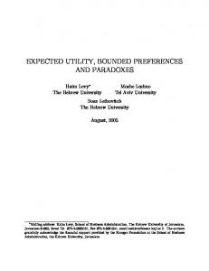
Figure 3: Construction of I1 , ..., I` m ≤ k. P P We would like to partition y∈Y km=1 vm`m(y) = 1 into ` portions so that each has the same sum 1` . However, this may not be directly possible; for example, if ` = 10 and v1 (y) = 2, 2 1 = 10 exceeds 1` = 10 . We avoid this by dividing vm`m(y) into `1m + ... + `1m . In Figure then v1`(y) 1 P P v1 (y) 3, is represented by 1, ..., τ 1 := y∈Y v1 (y) with weight `11 for each i = 1, ..., τ 1 . y∈Y `1 P In general, y∈Y vm`m(y) is represented by a set natural numbers Dm with weight `1m for each P P element in Dm . Thus, the set I = {1, ..., τ k } with τ k = km=1 y∈Y vm (y) is partitioned in D1 , ..., Dk with respect to the depths of associated weights. We partition this set I once more into I1 , ..., I` so that the summation of the weights over each It is 1` for t = 1, ..., `. Using these , ..., f`P ). two partitions, we construct f = (f1P Formally, let τ 0 = 0 and τ m = m y∈Y vd (y) for m = 1, ..., k. Then, let I = {1, ..., τ k }, d=1 and Dm = {τ m−1 + 1, ..., τ m } for m = 1, ..., k. We associate the weight w(i) to each i ∈ I by w(i) =
1 `m
if i ∈ Dm .
(45)
Each vm`m(y) is represented by the vm (y) number of elements in Dm associated with weights `1m . P P P P P P P Then, i∈Dm w(i) = y∈Y vm`m(y) , and km=1 i∈Dm w(i) = km=1 y∈Y vm`m(y) = y∈Y f (y) = 1. P Now, we define the function W over I by: W (j) = i≤j w(i) for any j ∈ I. Then, W (τ k ) = Pk P i∈Dm w(i) = 1. It holds that for any j ∈ I and t = 1, ..., `, m=1 t−1 `
≤ W (j)
1. The other case is |{i ∈ It ∩ D1 : ϕ(i) = y}| = 0. Hence, the summation in (48) has at most length k − 1. Then, since |{i ∈ It ∩ Dm : ϕ(i) = y}| ν for some ≤ |{i ∈ Dm : ϕ(i) = y}| = vm (y) < ` for all m ≤ k, the value ft (y) is expressed as `k−1 k−1 ν ≤ ` . Also, we have, by (47), P
ft (y) =
y∈Y
k |I ∩ D | k |{i ∈ I ∩ D : ϕ(i) = y}| P P P P t m t m = =`× w(i) = 1. m−1 m−1 ` ` m=1 y∈Y m=1 i∈It
Thus, ft ∈ Lk−1 (Y ) for all t = 1, ..., `. Finally,
¥
P`
1 t=1 `
× ft (y) is calculated as
` P k |{i ∈ I ∩ D : ϕ(i) = y}| k P ` |{i ∈ I ∩ D : ϕ(i) = y}| k v (y) P P P t m t m m = = = f (y). m m m ` ` t=1 m=1 m=1 t=1 m=1 `
References [1] Augustin, A., F. P. A. Coolen, G. de Cooman, M. C. T. Troffaes, (2014), Introduction to Imprecise Probabilities, Wiley, West Sussex. [2] Allais, M., (1953), Le comportement de l’homme rationnel devant le risque: critique des postulats et axiomes de l’ecole americaine, Econometrica 21, 503—546. [3] Anscombe, F. J., and R. J. Aumann, (1963), A Definition of Subjective Probability, Annals of Mathematical Statistics 34, 199-205. [4] Aumann, R. J., (1962), Utility Theory without the Completeness Axiom, Econometrica 30, 445—462. [5] Baucells, M., and L. S. Shapley, (2008), Multiperson Utility, Games and Economic Behavior 62, 329-347. [6] Blume, L. D. Easleya, and J. Y. Halpern, (2013), Constructive Decision Theory, Working Paper. [7] Hammond, P., (1998), Objective Expected Utility, Handbook of Utility Theory Vol.1: Principles, Ed. S. Barbera, et al. 143-211. [8] Dubra, J., F. Maccheroni, and E. A. Ok, (2004), Expected Utility Theory without the Completeness Axiom, Journal of Economic Theory 115, 118-133. [9] Galaabaatar, T., and E. Karni, (2013), Subjective Expected Utility with Incomplete Preferences, Econometrica 81, 255—284. 23
[10] Herstein, I. B. and J. Minor (1953), An Axiomatic Approach to Measurable Utility, Econometrica 21, 291-297. [11] Hu, T., (2013), Expected Utility Theory from the Frequentist Perspective, Economic Theory 53, 9—25. [12] Kahneman, D., and A. Tversky, (1979), Prospect Theory: An Analysis of Decision under Risk, Econometrica 47, 263-292. [13] Kaneko, M., and J. J. Kline, Inductive Game Theory: A Basic Scenario, Journal of Mathematical Economics 44, (2008), 1332—1363. [14] Kontek, K. and M. Lewandowski, Range-Dependent Utility, 2017, to appear in Management Science. http://www.mlewandowski.waw.pl/wp-content/uploads/2015/11/decision1.pdf [15] Nau, R., (2006), The Shape of Incomplete Preferences, The Annals of Statistics 34, 24302448. [16] Prelec, D. (1998), The Probability Weighting Function, Econometrica 60, 497-528. [17] Rubinstein, A., (1988), Similarity and Decision Making under Risk: Is there a Utility Theory Resolution to the Allais Paradox, Journal of Economic Theory 46, 145-153. [18] Savage, L. J., (1954), The Foundations of Statistics, John Wiley and Sons, New York. [19] Simon, H. A., (1956), Rational Choice and the Structure of the Environment, Psychological Review 63, 129—138. [20] Simon, H. A., (1983), Reason in Human Affairs, Stanford University Press, Stanford. [21] Tserenjigmid, G., (2015), Theory of Decisions by Intra-dimensional Comparisons, Journal of Economic Theory 159, 326-338. [22] Von Neumann, J., and O. Morgenstern, (1944), Theory of Games and Economic Behavior, 2nd ed. 1947, Princeton University Press, Princeton, N.J.
24