Exploiting Context for Semantic Scene Classification - UR Research

Exploiting Context for Semantic Scene Classification Matthew R. Boutell The University of Rochester Computer Science Department Rochester, New York 14627 Technical Report 894 2006

This research was supported by a grant from Eastman Kodak Company, by the NSF under grant number EIA0080124, and by the Department of Education (GAANN) under grant number P200A000306.

Exploiting Context for Semantic Scene Classification by Matthew R. Boutell

Submitted in Partial Fulfillment of the Requirements for the Degree Doctor of Philosophy Supervised by Professor Christopher M. Brown Dr. Jiebo Luo Department of Computer Science The College Arts and Sciences University of Rochester Rochester, New York 2005

iii

Dedication To my father, Robert Boutell, and my father-in-law Michael Preskenis, whose visions of Dr. Boutell continue to inspire me.

iv

Curriculum Vitae Matthew Richard Boutell was born on October 1, 1971 in Gardner, Massachusetts. A passion for math early in life led him to study at Worcester Polytechnic Institute. He first tasted the joys of research through a Research Experience for Undergraduates program and his senior project, both in graph theory, and graduated with a Bachelor of Science degree in Mathematical Science with high distinction in 1993. Putting his research interests temporarily on hold, the author earned a Master of Education degree from the University of Massachusetts, Amherst in 1994 and taught high school math and computer science at Norton (MA) High School for six years. During that time, he taught himself C++, leading to an internship as a software engineer and three semesters as an adjunct professor in the Computer Science department at Stonehill College in Easton, MA. He commenced graduate studies at the University of Rochester in 2000 and received the Master of Science degree in Computer Science in 2002. The author’s current research interests include computer vision, pattern recognition, probabilistic modeling, and image understanding.

v

Acknowledgments First and foremost, I would like to thank my co-advisors, Chris Brown and Jiebo Luo. Chris graciously took me under his wing after my first year. His availability to talk and listen was incredibly helpful − if I have abused that privilege at times, it is because I value his counsel. His words of encouragement have lifted me more than he probably realized. Jiebo has been a true mentor, teaching me daily the joys and heartbreaks of independent research. He has given me perseverance in the face of unexpected experimental results and harsh rejection letters from anonymous reviewers. He has been my closest collaborator and a fountain of ideas. I am grateful to the members of my thesis committee: Randal Nelson, Robbie Jacobs, and Ted Pawlicki for their questions and insights, and to Dan Gildea for timely clarification while I was writing this dissertation. Kevin Murphy inspired me to consider the dynamic factor graph framework. The vision and machine learning groups at Rochester have also been a great source of inspiration: Nathan Sprague, Manu Chhabra, Craig Harman, Jonathan Shaw, Phil Michalak, and many others. I enjoyed collaborating with several dedicated students in our department: Anustup Choudhury, Xipeng Shen, and Wenzhao Tan; each will each go far in his work. Anustup implemented the discriminative classifier appearing in Sections 5.5 and 5.6 and labored deep into the night running experiments for me. Thanks to Brian Madden for providing a fresh outlook on this work. I am grateful to Brandon Sanders for useful and inspiring discussions on statistical inference and Markov random fields. While we never got around to publishing our tech report, this dissertation serves as one of our desired “artifacts”. My fellow classmates made work fun along the journey: Bill Scherer, Andy Learn, Yutao Zhong, Tao Li, Qi Li, Proshanto Mukherji, and Samuel Chen. I will particularly miss Bill’s sensitivity and honest insights into our topics of conversation. The staff, Peg Meeker, Jo-Marie Carpenter, Eileen Pullara, Jill Forster, Marty Guenther, Elaine Heberle, Jim Roche, and Dave Costello, worked wonders to make sure I was registered, paid, insured, equipped, and wired while in the department. During the past four years, I sometimes worked as much on-site at Kodak as I did at the University, and am indebted to the past and present members of Kodak’s Image Understanding Working Group, Amit Singhal, Bob Gray, Wei Hao, David Crandall, and Rodney Miller, for ideas and encouragement. Finally, I thank my family for bearing with the long hours invested in this journey. Dad and Mom saw and grew this vision long before I did. Jonathan, Caleb, Elise, and Elliot, thank you for understanding when Daddy had to leave early and return home late while writing this “book”. Leah, thanks for enduring with the crazy schedules, being my biggest fan, and for helping in every way possible. You are the best. This research was supported by a grant from Eastman Kodak Company, by the NSF under grant number EIA-0080124, and by the Department of Education (GAANN) under grant number P200A000306.

vi

Table of Contents 1 2

Thesis Statement ......................................................................................................... 1 Introduction................................................................................................................. 2 2.1 Motivation........................................................................................................... 2 2.2 The Problem of Scene Classification.................................................................. 4 2.2.1 Scene Classification vs. Full-Scale Image Understanding ......................... 5 2.2.2 Scene Classification vs. Object Recognition .............................................. 5 2.3 Existing Work in Scene Classification ............................................................... 6 2.4 The Challenge of Consumer Photographs .......................................................... 6 2.5 Using Context in Scene Classification................................................................ 7 2.6 Graphical Models................................................................................................ 7 2.7 Contributions....................................................................................................... 8 3 Previous Work ............................................................................................................ 9 3.1 Scene Classification in the Literature ................................................................. 9 3.1.1 Design Space of Scene Classification......................................................... 9 3.1.2 Features ..................................................................................................... 10 3.1.3 Learning and Inference Engines ............................................................... 10 3.1.4 Scene Classification Systems.................................................................... 11 3.2 Use of Context in Intelligent Systems .............................................................. 18 3.2.1 Spatial Context.......................................................................................... 18 3.2.2 Temporal Context ..................................................................................... 18 3.2.3 Image Capture Condition Context ............................................................ 19 3.3 Graphical Models.............................................................................................. 19 3.3.1 Bayesian Networks ................................................................................... 20 3.3.2 Hidden Markov Models ............................................................................ 22 3.3.3 Markov Random Fields............................................................................. 25 3.3.4 Factor Graphs............................................................................................ 27 3.3.5 Belief Propagation in Factor Graphs......................................................... 28 3.3.6 Relative Merits of Each ............................................................................ 30 3.3.7 Why Generative Models? ......................................................................... 31 4 Content-based Classifiers.......................................................................................... 32 4.1 Low-level Features............................................................................................ 32 4.1.1 Spatial Color Moments for Outdoor Scenes ............................................. 32 4.1.2 Color Histograms and Wavelets for Indoor vs. Outdoor Classification ... 34 4.1.3 Support Vector Machine Classifier........................................................... 34 4.1.4 Limitations of Exemplar-based Systems .................................................. 35 4.1.5 Image-transform Bootstrapping ................................................................ 36 4.2 Semantic Features ............................................................................................. 38 4.2.1 Best-case Detectors (Hand-labeled Features) ........................................... 38 4.2.2 Actual Detectors........................................................................................ 40 4.2.3 Combining Evidence for a Region from Multiple Detectors.................... 41 4.2.4 Simulating Faulty Detectors for a Region ................................................ 43 5 Spatial Context.......................................................................................................... 46

vii 5.1 Semantic Features and Scene Classification..................................................... 46 5.2 Scene Configurations ........................................................................................ 47 5.2.1 Formalizing the Problem of Scene Classification from Configurations... 48 5.2.2 Learning the Model Parameters ................................................................ 49 5.2.3 Computing the Spatial Relationships........................................................ 49 5.3 Graphical Model ............................................................................................... 51 5.4 Factor Graph Variations for Between-Region Dependence ............................. 52 5.4.1 Exact ......................................................................................................... 52 5.4.2 Spatial Pairs.............................................................................................. 57 5.4.3 Material Pairs........................................................................................... 58 5.4.4 Independent............................................................................................... 58 5.5 Discriminative Approach to Using High-level Features................................... 59 5.6 Results and Discussion ..................................................................................... 60 5.6.1 Experimental Setup................................................................................... 60 5.6.2 Exact Scene Configuration Model ............................................................ 61 5.6.3 Spatial Pairs Scene Configuration Model ................................................ 63 5.6.4 Comparison between All Scene Classification Methods .......................... 65 5.7 Scene- and Spatially-aware Region Labeling ................................................... 68 5.7.1 Previous Work on Natural Object Detection ............................................ 68 5.7.2 Scene Context ........................................................................................... 69 5.7.3 Probabilistic Framework........................................................................... 70 5.7.4 Experimental Results ................................................................................ 71 5.8 Conclusions....................................................................................................... 72 6 Temporal Context ..................................................................................................... 74 6.1 Probabilistic Temporal Context Model............................................................. 75 6.2 Elapsed Time-dependent Transition Probabilities ............................................ 76 6.3 Learning ............................................................................................................ 77 6.3.1 Elapsed Time-dependent Transition Probabilities .................................... 77 6.3.2 Marginalized Transition Probabilities....................................................... 78 6.3.3 Output Probabilities .................................................................................. 79 6.4 Experimental Results ........................................................................................ 79 6.4.1 Problem 1: Indoor-outdoor Classification ................................................ 80 6.4.2 Problem 2: Sunset Detection..................................................................... 83 6.5 Conclusion and Future Work ............................................................................ 85 7 Image Capture Condition Context ............................................................................ 87 7.1 Digital Camera Metadata .................................................................................. 87 7.2 Families of Metadata Tags................................................................................ 88 7.3 Cue Selection Using Kullback-Leibler Divergence.......................................... 88 7.4 Cue Integration Using a Bayesian Network...................................................... 89 7.5 Indoor-Outdoor Classification .......................................................................... 90 7.5.1 KL Divergence Analysis........................................................................... 91 7.5.2 Cue Distributions for Indoor-Outdoor Images.......................................... 92 7.5.3 Experimental Results ................................................................................ 93 7.5.4 Simulating the Availability of Metadata................................................... 95 7.5.5 Discussions of Indoor-Outdoor Classification.......................................... 96 7.6 Sunset Scene Detection..................................................................................... 99

viii 7.7 Manmade-Natural Scene Classification.......................................................... 102 7.8 Conclusions..................................................................................................... 105 8 Conclusions............................................................................................................. 107 8.1 Limitations of the Current Work..................................................................... 108 8.2 Future Directions ............................................................................................ 108 8.2.1 Multilabel Scene Classification .............................................................. 109 8.2.2 Integrating Various Types of Context..................................................... 109 8.2.3 Partially-labeled Training Examples for Spatial Context ....................... 110 8.2.4 Geospatial Context for Scene Classification........................................... 110 8.2.5 User-specific Context Models................................................................. 111 8.2.6 Event-based Temporal Context............................................................... 111 9 Bibliography ........................................................................................................... 112 10 Appendix............................................................................................................. 123

ix

List of Tables Table 3.1. Options for features to use in scene classification........................................... 10 Table 3.2. Potential classifiers to use in scene classification............................................ 11 Table 3.3. Related work in scene classification, organized by feature type and use of spatial information........................................................................................................................ 13 Table 3.4. Sample transition probability matrix for indoor vs. outdoor scene classification. For example, when an image is of an outdoor scene, the probability the next image will be indoor is approximately 10%. .......................................................................................................... 23 Table 4.1. Likelihood vector for each region in Figure 4.7g. ........................................... 41 Table 4.2. Characteristics of sand detector. ...................................................................... 42 Table 5.1 Symbolic spatial arrangements and corresponding spatial relationships.......... 50 Table 5.2. Image sets used in Chapter 4. .......................................................................... 60 Table 5.3. Scene class descriptions................................................................................... 60 Table 5.4. Comparison between various techniques. SVMs with Gaussian kernels can be tuned to memorize their training sets, so the starred (*) entries would be meaningless. Accuracies (%) are shown. ............................................................................................................................... 64 Table 5.5. Comparison between techniques on D3. Accuracies (%) are shown. ............. 66 Table 5.6. Beach-specific pdf for B above A. ................................................................... 70 Table 5.7. Open-water-specific pdf for B above A. .......................................................... 70 Table 5.8. Improvement due to scene-context model (MAP) vs. two baselines: spatial-only context (MAPGen) and no context (MLE). ....................................................................... 72 Table 6.1. Elapsed-time dependent transition probabilities learned from data set D1. Note the trend towards the prior probability as elapsed time increases. ......................................... 80 Table 6.2. Transition probabilities learned from data set D1, marginalizing over elapsed time, for the order-only case............................................................................................................ 80 Table 6.3. Accuracy, in percent, of the elapsed-time dependent and independent context models using both inference schemes and three cross-validation methods. Both temporal models clearly outperform the baseline. Note that the margin of improvement induced by the elapsed time does not change over different cross-validation schemes. In addition, the differences in accuracy between the two inference algorithms are insignificant. Standard errors are shown in parentheses. ........................................................................................................................................... 81 Table 7.1. Statistical evidence for cues and cue combinations. The best results using one, two, and three cues are shown in boldface. .............................................................................. 91 Table 7.2. Distribution of flash in indoor and outdoor scenes.......................................... 93 Table 7.3. Accuracy using metadata cues and combinations............................................ 93 Table 7.4. Accuracy when low-level cues are added........................................................ 94 Table 7.5. Performance when simulating incomplete metadata cues. .............................. 96 Table 7.6. Number of images in each category from D1.................................................. 96 Table 8.1. Potential presentation orders for the context types........................................ 107

x

List of Figures Figure 2.1. Querying an image database by color only sometimes gives understandable, but unmeaningful results. Here, a query for a Ferrari can return a rose if the two images are most similar in global color distributions. ................................................................................... 3 Figure 2.2. Image retrieval aided by off-line classification. Annotating images belonging to the car class enables us to search only that subset, leading to more accurate, more efficient results. Here, the same query for a Ferrari yields another Ferrari, as expected. ............................. 3 Figure 2.3. Attempting to color-balance a sunset scene is undesirable, removing brilliant colors. (Left) The original image. (Center) After generic enhancement. (Right) After sunset-aware enhancement. ...................................................................................................................... 4 Figure 3.1. A Bayes Net with a loop................................................................................. 21 Figure 3.2. An appropriate graphical model for temporally related images is a Hidden Markov Model. The C nodes (class) are the hidden states and the E nodes (evidence) are the observed states.................................................................................................................................. 22 Figure 3.3. A portion of the trellis obtained by unwrapping the hidden Markov model over time to show the potential sets of states. See text for details. ................................................... 24 Figure 3.4. Portion of a typical two-layer MRF. In low-level computer vision problems, the top layer (black) represents the external evidence of the observed image while the bottom layer (white) expresses the apriori knowledge about relationships between parts of the underlying scene.................................................................................................................................. 26 Figure 3.5. An example of a tree structured factor graph. Both graphs are equivalent, but the one on the right is visualized as sets of variables and factors, accentuating the bipartite nature of the graph. ................................................................................................................................ 28 Figure 4.1. Spatial color moment features. ....................................................................... 33 Figure 4.2. Choosing an optimal hyperplane. The circled points lying on the margin (solid lines) are the support vectors; the decision surface is shown as a dotted line. The hyperplane on the right is optimal, since the width of the margin is maximized. Note that with separable data, there is no need to project it to a higher dimension. .................................................................. 35 Figure 4.3. “Reliving the scene”. The original scene (a) contains a salient subregion (b), which is cropped and resized (c). Finally, an illuminant shift (d) is applied, simulating a sunset occurring later in time. ...................................................................................................................... 36 Figure 4.4. Screenshot of our labeling utility. The image is segmented using a general purpose segmentation algorithm, then the semantically-critical regions are labeled interactively. In this screenshot, the foliage and pavement are labeled so far................................................... 39 Figure 4.5. Process of hand-labeling images (a) A street scene. (b) Output from the segmentation-based labeling tool. (c) Output from a manmade object detector. (d) Combined output, used for learning spatial relation statistics............................................................ 39 Figure 4.6. Process of material detection, shown for the foliage detector. (a) Original image (b) Pixel-level belief map. (c) Output of individual detector. In (b) and (c), brightness corresponds to belief values. ..................................................................................................................... 40 Figure 4.7. Aggregating results of individual material detectors for an image (a) Original image (b)-(f) are individual detectors: (b) Blue-sky (c) Cloudy sky (d) Grass (e) Manmade (f) Sand. The foliage detection result from Figure 4.6 is also used. Other detectors gave no response. (g) The aggregate image. Brightness of its 7 detected regions ranges from 1 (darkest non-black region) to

xi 7 (brightest). The corresponding beliefs for each region are given in Table 4.1. (h) Pseudocolored aggregate image. .................................................................................................. 41 Figure 4.8. Bayesian network subgraph showing relationship between regions and detectors. ........................................................................................................................................... 42 Figure 5.1 (a) A beach image (b) Its manually-labeled materials. The true configuration includes sky above water, water above sand, and sky above sand. (c) The underlying graph showing detector results and spatial relations. ................................................................................ 47 Figure 5.2. Common factor graph framework for scene classification. The actual topology of the network depends on the number of regions in the image and on the independence assumptions that we desire (see text for details). .................................................................................. 52 Figure 5.3. Factor graph for full scene configuration (n = 3 regions). Due to its tree structure, we can perform exact inference on it. However, the complexity of the model is hidden in the spatial configuration factor; learning it is problematic. ............................................................... 53 Figure 5.4. Options for smoothing the sparse distribution. For clarity, we only show a two dimensional distribution and training examples falling into two bins (shown as vertical lines). ........................................................................................................................................... 54 Figure 5.5. Smoothing in two and three dimenstions. On the left, an example in the position (2,5) contributes 1 to the count in that position and because the “subgraphs” are 2 and 5, it contributes ε to the counts in (n,2), (2,n), (n,5), and (5,n). The figure on the right is explained in the text. For legibility in this 3D example, only one training point and two backprojection directions (of the three possible with this spatial configuration) are shown................................................. 55 Figure 5.6. Factor graph for scene configuration (n = 3 regions), approximated using pairwise spatial relationships. While it is not exact due to the loops, each spatial factor’s parameters are easier to learn than the joint one proposed in Figure 5.3. Furthermore, its dynamic structure allows it to work on any image. ........................................................................................ 58 Figure 5.7. Factor graph assuming regions are independent. This is equivalent to a tree-structured Bayesian network.............................................................................................................. 59 Figure 5.8. Classification accuracy of the methods as a function of detector accuracy. The subgraph-based smoothing method performs better than the baselines at nearly all detector accuracies. Standard error is shown (n = 30). .................................................................. 62 Figure 5.9. Some images for which the baseline smoothing methods fail, but the subgraph-based method succeeds. Top: original scenes. Bottom: hand-labeled regions. .......................... 63 Figure 5.10. Classification accuracy of the methods as a function of simulated detector accuracy. We repeated each simulation 10 times and report the mean accuracy. The standard deviation between test runs is extremely small (standard error is negligible).................................. 64 Figure 5.11. Comparison between accuracy obtained using the Spatial Pairs model (and variations explained in text), the Exact model, and the discriminative model using high level features for the range of simulated detector accuracy. ..................................................... 67 Figure 5.12. Architecture of a holistic object-detection system. ...................................... 69 Figure 5.13. The material pdfs just described are 2D slices of the factors of Spatial Pairs.71 Figure 5.14. A field example showing improvement due to scene-specific spatial model over both baselines.................................................................................................................... 72 Figure 6.1. Transition function for P (C i = cˆ | C i −1 = cˆ, τ ) . The horizontal asymptote is the prior probability, P(Ci = cˆ ) . ........................................................................................... 77

xii Figure 6.2. Elapsed time-dependent temporal context model. The transition probabilities used between two images are a function of the elapsed time between them. As τÆ τn, the probabilities approach the class priors................................................................................................... 78 Figure 6.3. Comparison of the baseline content-based indoor-outdoor classifier with those improved by the temporal models (with and without elapsed time). Note that this is not a typical ROC curve because we want to show the balance between accuracy on each of the two classes. ........................................................................................................................................... 82 Figure 6.4. Image sequences affected by the context model. Elapsed times (in seconds) between images are shown. The first three sequences show examples in which the model corrected errors made by the baseline classifier. The fourth sequence shows a conceptual error: a rare case where the photographer walks into a room briefly between taking two outdoor photos. The last two sequences show examples where long elapsed time causes no change. ........................... 83 Figure 6.5. Comparison of baseline content-based sunset detector performance with those improved by the temporal context models, with and without elapsed time. For any false positive rate, the recall of sunsets can be boosted by 2-10%. Alternately, for a given recall rate, the false positive rate can be reduced by as much as 20% in high recall operating points. ............ 84 Figure 6.6. Two sunset image sequences affected by the context model. In each case, the model corrects an error. The first sequence is typical: indoor images under low incandescent lighting can often be confused as sunsets, but are easy to correct by the temporal model. The second sequence shows a burst of sunset images in which two “weak” (cool-colored) sunsets are missed by the color-texture classifier, but corrected by the model............................................... 85 Figure 7.1. Bayesian network for evidence combination. ................................................ 90 Figure 7.2. Distribution of exposure times (ET) of indoor and outdoor scenes. .............. 92 Figure 7.3. Distribution of subject distance (SD) of indoor and outdoor scenes.............. 92 Figure 7.4. Comparison of individual metadata cues. ...................................................... 94 Figure 7.5. Comparison of performance using low-level, metadata, and combined cues. LL = low-level, FF = flash fired, ET = exposure time, SD = subject distance. Note that the image capture condition cues alone outperform image data alone, but that the combination of the two cue types yields the highest performance. ........................................................................ 95 Figure 7.6. Indoor image samples, classified correctly by both (row 1), gained by metadata (row 2), lost by metadata (row 3), and incorrectly regardless of cues (row 4). ........................ 97 Figure 7.7. Outdoor image samples, classified correctly by both (Row 1), gained by metadata (Row 2), lost by metadata (Row 3), and incorrectly regardless of cues (Row 4)............. 98 Figure 7.8. Distributions of beliefs for indoor and outdoor scenes in D1 shows that belief is an accurate measure of confidence. ....................................................................................... 99 Figure 7.9. Accuracy vs. rejection rate obtained by thresholding the final beliefs........... 99 Figure 7.10. Performance of content-only vs. metadata-enhanced sunset detection. As an example, at the 0.5 threshold, sunset recall rose from 79.6% to 94.8%, while the false positive rate dropped slightly from 6.0% to 5.5%........................................................................ 100 Figure 7.11. Sunset image samples, classified correctly by both (row 1), gained by metadata (row 2), lost by metadata (row 3), and incorrectly regardless of cues (row 4). Only a single sunset image was lost by metadata. ........................................................................................... 101 Figure 7.12. Non-sunset image samples, classified correctly by both content-based and combined cues (row 1), gained by metadata (row 2), lost by metadata (row 3), and incorrectly regardless of cues (row 4)..................................................................................................................... 102

xiii Figure 7.13. Performance of content-only vs. metadata-enhanced manmade-natural image classification. Metadata improved accuracy across the entire operating range (average +2%). ......................................................................................................................................... 103 Figure 7.14. Manmade image samples, classified correctly by both content-based and combined cues (row 1), gained by metadata (row 2), lost by metadata (row 3), and incorrectly regardless of cues (row 4)..................................................................................................................... 104 Figure 7.15. Natural image samples, classified correctly by both content-based and combined cues (row 1), gained by metadata (row 2), lost by metadata (row 3), and incorrectly regardless of cues (row 4)..................................................................................................................... 105 Figure 8.1. Multilabel images. The image on the left is both a beach scene and an urban scene, while the one on the right is both a field scene and a mountain scene. .......................... 109

xiv

Abstract Semantic scene classification, automatically categorizing images into a discrete set of classes such as beach, sunset, or field, is a difficult problem. Current classifiers rely on low-level image features, such as color, texture, or edges, and achieve limited success on constrained image sets. However, the domain of unconstrained consumer photographs requires the use of new features and techniques. One source of information that can help classification is the context associated with the image. We have explored three types of context. First, spatial context enables the use of scene configurations (identities of regions and the spatial relationships between the regions) for classification purposes. Second, temporal context allows us to use information contained in neighboring images to classify an image. We exploit elapsed time between images to help determine which neighboring images are most closely related. Third, image capture condition context in the form of camera parameters (e.g., flash, exposure time, and subject distance) recorded at the time the photo was taken provides cues that are effective at distinguishing certain scene types. We developed and used graphical models to incorporate image content with these three types of context. These systems are highly modular and allow for probabilistic input, output, and inference based on the statistics of large image collections. We demonstrate the effectiveness of each context model on several classification problems.

1

1 Thesis Statement Classification of images, consumer photographs in particular, is a difficult problem. Existing approaches rely on low-level features such as color, texture, and edges, and use techniques from statistical pattern recognition to separate the image classes in the feature space. We believe that advances to the state of the art must be made outside of this typical scheme of low-level features + classifier du jour. The thesis put forth in this dissertation is that incorporating context can help to classify scenes. This context can take on many forms. One powerful and better-known type of context is the set of keywords stored in the camera metadata that photographers have entered to label their images. However, entering keywords manually can be a tedious task, and so is rarely performed, except in certain image and video domains (e.g., network news clips). In this dissertation, we explore three other types of image context: Spatial context. Object detectors can find various components, such as sky, buildings, grass, or pavement, within photographs with some success. The presence alone of certain objects provides some evidence as to the type of scene (e.g., sky, water, and sand in a beach scene); however, the configurations of these objects, including their spatial relationships, can provide more reliable information, and help correct errors made by the detectors. Temporal context. Because photographers take photos to tell stories, photographs are related to adjacent ones. Our temporal context model using timestamps exploits the fact that the correlation between two images increases as the elapsed time between them decreases. However, the model is general enough to work in situations where the elapsed times are unknown (film scans) or fixed (video). Image capture condition context. In the header of all JPG image files, cameras record metadata such as the exposure time, subject distance, and flash fire. This information provides effective cues to discriminate certain scene classes (e.g., sunset, indoor vs. outdoor). Each of these three types of context can be extracted from the image or collection without additional manual labor. In each case, we combine the context cues with the image content using a probabilistic graphical model (e.g., Bayesian network, factor graph, hidden Markov model). We learn the context cue parameters from large image databases, as opposed to following handcoded rules. One advantage of probabilistic models is that the final belief value in a classification can be used as a measure of confidence to rank the images, to determine if a human should examine them, or to facilitate their combination with additional cues. Because they are generative models, they serve a general purpose, work relatively well when the training set is small, and can function in the presence of missing data. Finally, they are also modular, so improved components can be incorporated without retraining the entire system. This modularity is important in a large research setting in which the system is too large to be designed quickly by a single researcher.

2

2 Introduction In which we define scene classification, differentiating it from image processing and full image understanding, present a number of applications which could benefit from it, constrain our domain to consumer photography, and propose the use of context.

Semantic scene classification is defined as the process of automatically categorizing images into a discrete set of semantic classes such as indoor vs. outdoor, manmade vs. natural, or beaches vs. sunsets vs. mountains. As humans, we can quickly determine the classification of a scene, even without recognizing every detail present. Even the gist of a scene communicates much. The utility of scene classification continues to increase in the current age of electronic media.

2.1 Motivation With digital image libraries growing in size so quickly, accurate and efficient techniques for image organization and retrieval become more and more important. Automatic semantic classification of digital images finds many applications. We describe three major ones briefly: content-based image organization, content-based image retrieval (CBIR) and content-sensitive digital enhancement. First, scene classification can be used directly to organize photographs. For example, outdoor images form a cluster and within that cluster, sunsets, fields, and beach scenes form subclusters. Hierarchical methods have been proposed [Vailaya et al., 1999a; Lim et al., 2003]. Second, scene classification can improve CBIR systems. These systems allow a user to specify an image and then search for images similar to it, but similarity is often defined only by color or texture properties. Because a score is computed on each image in the potentially-large database, it is somewhat inefficient (though individual calculations vary in complexity). Furthermore, this so-called “query by example” has often proven to return inadequate results [Smeulders et al., 2000]. Sometimes the match between the retrieved and the query images is hard to understand, while other times, the match is understandable, but contains no semantic value. For instance, with simple color features, a query for a red sports car can return a picture of a rose, especially if the background colors are similar as well (Figure 2.1). Knowledge of scene classes helps narrow the search space dramatically [Luo and Savakis, 2001]. If the categories of the query image and the database images have been assigned off-line, either manually or by an algorithm, a system can exploit them at search time to improve both efficiency and accuracy.

3

Query

Database

Result

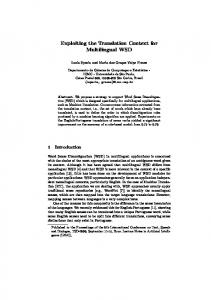
Figure 2.1. Querying an image database by color only sometimes gives understandable, but unmeaningful results. Here, a query for a Ferrari can return a rose if the two images are most similar in global color distributions. Above, if the car scenes could be recognized and labeled, then a query for a car would only search within the subset of images belonging to that class (Figure 2.2). This approach would reduce the search time, increase the hit rate, and lower the false alarm rate. In another realistic example, knowing what constitutes a beach scene would allow us to consider only beach scenes in our query, find photos of John on the beach. Vailaya [2000] shows additional examples.

Class: CAR

CAR

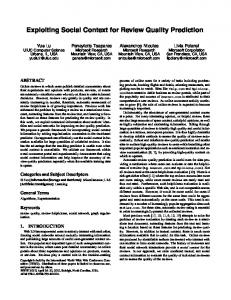
Figure 2.2. Image retrieval aided by off-line classification. Annotating images belonging to the car class enables us to search only that subset, leading to more accurate, more efficient results. Here, the same query for a Ferrari yields another Ferrari, as expected. Third, understanding an image’s content can automate manual steps in the process of digital image enhancement. For example, Ofoto, a leading online digital photo service, must crop

4 images in which the aspect ratio of the capture device and the print medium are different (e.g., from 4:3 to 3:2). One of the most conspicuous cropping errors is removing the top of a person’s head. To reduce the probability of this happening, an automatic algorithm uses location of the image’s main subject, usually a person [Singhal, 2001], as part of its determination of where to crop the image [Luo and Gray, 2003]. As a second example, digital images are often oriented incorrectly when captured, either by a camera, when it is held sideways to take a portrait, or by a scanner when the image is placed sideways. They must then be re-oriented manually for displaying on computers, televisions, or handheld devices. An automatic algorithm for recognizing mis-oriented images and re-orienting them to the upright position can reduce much of the tedious labor involved. Knowledge of a scene’s class can also allow for content-sensitive digital enhancement [Szummer and Picard, 1998]. Digital photofinishing processes involve three steps: digitizing the image (if the original source was film), applying enhancement algorithms, and outputting the image in either hardcopy or electronic form. Enhancement consists primarily of color balancing, exposure enhancement, and noise reduction. Currently, enhancement operates without knowledge of the scene content. Unfortunately, while a generic balancing algorithm might enhance the quality of some classes of pictures, it degrades others. Take color balancing as an example. Photographs captured under incandescent lighting without flash tend to be yellowish in color. Color balancing removes the yellow cast. However, when a generic algorithm applies the same color balancing to a sunset image, which contains the same yellowish global color distribution, it can destroy the desired brilliance (Figure 2.3b).

Figure 2.3. Attempting to color-balance a sunset scene is undesirable, removing brilliant colors. (Left) The original image. (Center) After generic enhancement. (Right) After sunset-aware enhancement. Other images affected negatively by color balancing are those containing colors resembling skin tones. Correctly balanced skin colors are important to human perception [Semba et al., 2001], and it is important to balance them. However, causing non-skin objects with similar colors to look like skin is a conspicuous error. Rather than applying generic color balancing and exposure adjustment to all images, knowledge of the scene's semantic classification allows us to customize them to the scene. Following the example above, we could retain or even boost sunset scenes' brilliant colors (Figure 2.3c) while reducing a tungsten-illuminated indoor scene's yellowish cast.

2.2 The Problem of Scene Classification On one hand, isn't scene classification preceded by image understanding, the “holy grail” of vision? What makes us think we can achieve results? On the other hand, isn't scene classification just an extension of object recognition, for which many techniques have been proposed with varying success? How is scene classification different from these two related fields?

5

2.2.1 Scene Classification vs. Full-Scale Image Understanding As usually defined, image understanding is the process of converting “pixels to predicates”: (iconic) image representations to another (symbolic) form of knowledge [Ballard and Brown, 1982]. Image understanding is the highest processing level in computer vision [Sonka et al., 1999], as opposed to image processing techniques, which convert one image representation to another. For instance, converting raw pixels to edgels using a linear shift-invariant operator is a lower and earlier operation than identifying the expression on a person's face in the image. Lower-level image processing techniques such as segmentation are used to create regions that can then be identified as objects. Various control strategies are used to order the processing steps and can vary [Batlle et al., 2000; Rimey, 1993]. The end result desired is for the vision to support high-level reasoning about the objects and their relationships to meet a goal. While image understanding in unconstrained environments is still very much an open problem [Sonka et al., 1999; Vailaya et al., 1999a], much progress is currently being made in scene classification. Because scenes can often be classified without full knowledge of every object in the image, the goal is not as ambitious. For instance, if a person recognizes trees at the top of a photo, grass on the bottom, and people in the middle, he may hypothesize that he is looking at a park scene, even if he cannot see every detail in the image. Or on a different level, if he sees many sharp vertical and horizontal edges, he may be looking at an urban scene. It may be possible in some cases to use low-level information, such as color or texture, to classify some scene types accurately. In other cases, object recognition may be necessary, but not necessarily of every object in the scene. In general, classification seems to be an easier problem than unconstrained image understanding; early results have confirmed this for certain scene types in constrained environments [Torralba and Sinha, 2001b; Vailaya et al., 1999a]. Scene classification is a subset of the image understanding problem, and can be used to ease other image understanding tasks [Torralba and Sinha, 2001a]. For example, knowing that a scene is of a beach constrains where in the scene one should look for people. Obtaining full-scale image understanding in unconstrained environments is a lofty goal, and one worthy of pursuit. However, given the state of image understanding, we see semantic scene classification as a necessary stepping-stone in pursuit of the “holy grail”.

2.2.2 Scene Classification vs. Object Recognition However, scene classification is a different beast than object recognition. Detection of rigid objects can rely upon geometrical relationships within the objects. Various techniques [Forsyth et al., 1991; Selinger and Nelson, 1999] can achieve invariance to affine transforms and changes in scene luminance. Some object recognizers attempt to infer a full 3D model, while others use a 2D appearance model; in either case, hypothesized objects (or features from them) are matched against a canonical object (or set of such objects) or object views. Detection of non-rigid objects is less constrained physically, since the relationships are looser [Chang and Krumm, 1999]. Scene classification is even less constrained, since the components of a scene are varied. For instance, while humans might find it easy to recognize a scene of a child's birthday party, the objects and people that populate the scene can vary widely. The cues that determine the birthday scene class can be subtle − consider special decorations, articles marked with the age of the child, and facial expressions on the attendees. Even the more obvious cues, like a birthday cake, may be difficult to recognize.

6 Again, scene classification and object recognition are related; knowing the identity of some of the scene's objects will certainly help to classify the scene, while knowing the scene type affects the expected likelihood and location of the objects it contains. We now study current techniques for scene classification.

2.3 Existing Work in Scene Classification Most current scene classification systems rely on low-level features and achieve some success on constrained problems; we describe a few representative systems in Section 3.1. These systems are usually exemplar-based, in which features are extracted from images and pattern recognition techniques are used to learn the statistics of a training set and to classify novel test images. Unfortunately, these systems can often be plagued by a shortage of labeled training data. We use such a system as a baseline (Chapter 4), and introduce the concept of image-transform bootstrapping, an appealing idea we thoroughly explored that can help compensate for a shortage of data.

2.4 The Challenge of Consumer Photographs The domain of photography poses a large challenge to semantic scene classification. First, photographs of naturally-occurring scenes are much less constrained than those of experimental environments. We cannot fix illumination, pose, or any other variable, but must cope with the general content, mistakes, and vagaries of real photos. Second, our specific domain is home (or consumer) photography, most of which was captured by amateurs. Most scene classification systems (e.g., [Vailaya et al., 2002; Smith and Li, 1999]) reported success on professionally-photographed image sets, such as Corel. Major differences exist between Corel stock photos and typical consumer photos [Segur, 2000], including but not limited to the following: 1. Corel images used by Vailaya, et al. [2002] are predominantly outdoor and frequently with sky present, while there are roughly equal numbers of indoor and outdoor consumer pictures. 2. More than 70 percent of consumer photos contain people, opposite that of Corel photos. 3. Corel photos of people are usually portraits or pictures of a crowd, while in consumer photos the typical subject distance is 4-10 feet (thus, containing visible, yet not dominating, faces). 4. Consumer photos usually contain a much higher level of background clutter. 5. Consumer photos vary more in composition because the typical amateur pays less attention to composition and lighting than would a professional photographer, causing the captured scene to look less prototypical and thus not match any of the training exemplars well. 6. From a technical standpoint, the structure of the Corel library (100 related images per CD) often leads to some correlation between training and testing sets.

7 These differences cause many systems’ high performance on clean, professional stock photo libraries to decline markedly because it is difficult for exemplar-based systems to account for such variation in their training sets; analysis of consumer snapshots demands a more sophisticated approach. Most of our experiments are carried out on consumer images. The only exceptions are some of the outdoor image classes, for which it was far easier to obtain training data from the Corel collection due to its structure.

2.5 Using Context in Scene Classification Scene classification based on image content alone is an interesting problem, and there is still much room for improvement in techniques that use content only. However, my thesis is that various forms of context can help improve scene classification as well. In this dissertation, I define context broadly to include the following: With respect to region-based features such as detected materials or objects, I define the spatial context of a region to be the identities of other regions in the image and the spatial relationships between the regions. These may be coarse grained (e.g., above, beside, enclosed) or fine-grained (e.g., 56 pixels away at a bearing of 48 degrees). I use spatial context when modeling scene configurations, described in Chapter 5. Spatial context is perhaps the most narrow type of context, as it relates parts of a single image. With respect to image collections, an image’s temporal context includes those images that are temporally adjacent to it. Because photographers take pictures to tell a story, we expect these neighboring images, and thus their classifications, to be related. Chapter 6 details our temporal context model that exploits the information contained in the elapsed time between images. Temporal context is broader than spatial context, as it encompasses multiple images. Finally, digital images contain embedded metadata recorded by the camera about the conditions at the time the image was captured. These include whether the flash fired, the exposure time, the aperture value, the subject distance, and many other fields. This image capture context, described in Chapter 7, provides scene cues complementary to the image content for discriminating between certain scene types. Image capture context is perhaps broadest of all these types, not even relying on a single pixel in the image collection (albeit referring to a single image at a time). We note that multiple types of context can be integrated, but in this work, we study each of them independently.

2.6 Graphical Models For each of the preceding types of context, we integrate contextual cues with local content using a probabilistic framework. Graphical models are a convenient way to represent independence assumptions in the model. Furthermore, we model the relationship between the image and its class using generative models. Generative models are a parameterized probabilistic model of the joint distribution between all variables: input (image) and output (scene class). The graphical models we used, Bayesian networks, hidden Markov models, and factor graphs, are all generative models, as opposed to discriminative models, e.g., conditional random fields [Lafferty et al., 2001; Kumar and Hebert, 2003]. We use them to estimate or maximize the posterior probability (given an image or sequence of images) of the model parameters (e.g., the scene class). One distinction between generative and discriminative models is that one can sample from

8 generative models (e.g., mixture of Gaussians) but not from a discriminative model (e.g., neural network). We give an overview of graphical models in Section 3.3 and describe the particular models used in our work in Chapters 5-7.

2.7 Contributions In this work, we have made a number of technical contributions, summarized here. 1. Working scene classification system combining object detection and explicit spatial relations using a dynamic graphical model with spatial relation factors (Section 5.4) [Boutell et al., 2004a]. 2. Working scene classification system combining object detection and implicit spatial relations, found by extracting features using a block-based scheme (Section 5.5) [Boutell et al., 2005a]. 3. First classification system for image collections using timestamp-based temporal context (Chapter 6) [Boutell and Luo, 2004b; Boutell et al., 2005c]. 4. First classification system for image collections using image capture context (Chapter 7) [Boutell and Luo, 2004a; Boutell and Luo, 2005]. 5. General factor-graph framework able to handle different amounts of spatial context: full joint distribution of scene configurations, pairwise spatial relations, and pairwise co-occurance relations (Sections 5.3 and 5.4). 6. Framework for improving material detection based on knowledge of scene type and spatial relationships (Section 5.7) [Boutell et al., 2005b ]. 7. Framework for using image transforms to improve exemplar-based scene classifiers by populating the feature space more densely in training and increasing matches in testing (Section 4.1.5) [Boutell et al., 2003; Luo et al., 2005b].

9

3 Previous Work In which the literature gives us a starting point by providing answers to three questions. First, what has been done in scene classification? Second, how has context been exploited in artificial intelligence applications? Third, why use probabilistic approaches and graphical models in particular?

The material in Section 3.1 was taken in part from our review of the state of the art in scene classification [Boutell et al., 2002] referenced in our preliminary work [Boutell, 2005], while Section 3.3 was taken from the preliminary work [Boutell, 2005].

3.1 Scene Classification in the Literature Scene classification is a young, emerging field. We focus our attention on systems using approaches directly related to this thesis and appearing in our review [Boutell et al., 2002], to which we refer readers desiring a more comprehensive survey or more detail. All systems classifying scenes must extract appropriate features and use some sort of learning or inference engine to classify the image. We start by outlining the options available for features and classifiers. We then present a number of systems which we have deemed to be good representatives of the field.

3.1.1 Design Space of Scene Classification The literature reveals two approaches to scene classification: exemplar-based and model-based. On one hand, exemplar based approaches use pattern recognition techniques on vectors of lowlevel image features (such as color, texture, or edges) or semantic features (such as sky, faces or grass). The exemplars are thought to fall into clusters, which can then be used to classify novel test images, using an appropriate distance metric. Most systems use an exemplar-based approach, perhaps due to recent advances in pattern recognition techniques. On the other hand, modelbased approaches are designed using expert knowledge of the scene such as the expected configuration of a scene. A scene's configuration is the layout (relative location and identities) of its objects. While it seems as though this should be very important, relatively little research has been done on developing such systems to classify photographs (as opposed to objects in photographs). In either case, appropriate features must be extracted for accurate classification. What makes a certain feature appropriate for a given task? For pattern classification, one wants the inter-class distance to maximized and the intra-class distances to be minimized. Many choices are intuitive, e.g. edge features should help separate city and landscape scenes [Vailaya et al., 1998].

10

3.1.2 Features In our review [Boutell et al., 2002], we described features we found in similar systems, or which we thought could be potentially useful. Table 3.1 is a summary of that set of descriptions. Table 3.1. Options for features to use in scene classification. Feature Description Color Histograms[Swain and Ballard, 1991], Coherence vectors [Pass et al., 1996], Moments [Vailaya et al., 2002] Texture [Randen and Wavelets [Mallat, 1989; Serrano et al., 2004], MSAR [Szummer Husoy, 1999] and Picard, 1998], Fractal dimension [Sonka et al., 1999] Filter Output Fourier & discrete cosine transforms [Oliva and Torralba, 2001; Szummer and Picard, 1998; Torralba and Sinha, 2001a; Torralba and Sinha, 2001b; Vailaya et al., 1999a], Gabor [Schmid, 2001], Spatio-temporal [Rao and Ballard, 1997] Edges Direction histograms[Vailaya et al., 1999a], Direction coherence vectors [Vailaya et al., 1999a] Context Patch Dominant edge with neighboring edges [Selinger and Nelson, 1999] Object Geometry Area, Eccentricity, Orientation [Belongie et al., 1997] Object Detection Output from belief-based material detectors [Luo et al., 2003a; Singhal et al., 2003], rigid object detectors [Selinger and Nelson, 1999], face detectors [Schneiderman and Kanade, 2000] IU Output Output of other Image Understanding systems, e.g., main subject detection [Singhal, 2001] Mid-level “Spatial envelope” features [Oliva and Torralba, 2002] Statistical Measures Dimensionality reduction [Duda et al., 2001, Roweis and Saul, 2000]

3.1.3 Learning and Inference Engines Pattern recognition systems classify samples represented by feature vectors (for a good review, see [Jain et al., 2000]). Features are extracted from each of a set of training images, or exemplars. In most classifiers, a statistical inference engine then extracts information from the processed training data. Finally, to classify a novel test image, the system extracts the same features from the test image and compares them to those in the training set [Duda et al., 2001]. Various classifiers differ in how they extract information from the training data. Most current systems use this exemplar-based approach. In Table 3.2, we present a summary of the major classifiers used in the realm of scene classification.

11

Table 3.2. Potential classifiers to use in scene classification. Classifier Description 1-Nearest-Neighbor (1NN) Classifies test sample with same class as the exemplar closest to it in the feature space according to some distance metric, e.g., Euclidean. K-Nearest-Neighbor (kNN) [Duda et al., Generalization of 1NN in which the sample 2001] is given the label of the majority of the k closest exemplars. Learning Vector Quantization (LVQ) A representative set of exemplars, called a [Kohonen, 1990; Kohonen et al., 1992] codebook, is extracted. The codebook size and learning rate must be chosen in advance. Mixture of Gaussians [Vailaya et al., Models the class likelihoods modeled with 1999a] a mixture of Gaussians, each centered at a codebook vector (learned with LVQ) and weighted by the number of exemplars mapped to that vector. Support Vector Machine (SVM) [Burges, Find an optimal hyperplane separating two 1998; Scholkopf et al., 1999] classes. Maps data into higher dimensions, using a kernel function, to increase separability. The kernel and associated parameters must be chosen in advance. Artificial Neural Networks (ANN) Function approximators in which the inputs [Ballard, 1997] are mapped, through a series of linear combinations and non-linear activation functions to outputs. The weights are learned using backpropagation.

3.1.4 Scene Classification Systems As stated, many of the systems proposed in the literature for scene classification are exemplarbased, but a few are model-based, relying on expert knowledge to model scene types, usually in terms of the expected configuration of objects in the scene. In this section, we describe briefly some of these systems and point out some of their limitations en route to differentiating our model-based method. We organize the systems by feature type and in the use of spatial information, as shown in

12 Table 3.3. Features are grouped into low-level, mid-level, and high-level (semantic) features, while spatial information is grouped into those that model the spatial relationships explicitly in the inference stage and those that do not.

13

Table 3.3. Related work in scene classification, organized by feature type and use of spatial information. Spatial Information Feature Type Implicit/None Explicit Low-level Vailaya, et al, Oliva, et al., Szummer & Lipson, et al., Ratan & Picard, Serrano, et al., Paek & Chang, Grimson, Smith & Li Belongie, et al., Wang, et al.. Mid-level Oliva, et al. High-level Luo, et al., Song & Zhang Mulhem, et al., (semantic) Our method 3.1.4.1 Low-level Features and Implicit Spatial Relationships A number of researchers have used low-level features sampled at regular spatial locations (e.g. blocks in a rectangular grid). In this way, spatial features are encoded implicitly, since the features computed on each location are mapped to fixed dimensions in the feature space. The problems addressed by others include indoor vs. outdoor classification [Szummer and Picard, 1998; Paek and Chang, 2000; Serrano et al., 2004], outdoor scene classification [Vailaya et al., 1999a], and image orientation detection [Vailaya et al., 2002; Wang and Zhang, 2004] (While image orientation detection, determining which of the four compass directions is the top of the image, is a different level of semantic classification, many of the techniques used are similar.) The indoor vs. outdoor classifiers’ accuracy reported in the literature approaches 90% on consumer image sets when independent training and testing sets are drawn from the same source. On the outdoor scene classification problem, mid-90% accuracy is reported. This may be due to the use of constrained data sets (e.g. from the Corel stock photo library), because on less constrained (e.g., consumer) image sets drawn from different sources, we found the results to be lower. The generalizability of the technique is also called into question by the discrepancies in the numbers reported for image orientation detection by some of the same researchers [Vailaya et al., 2002; Wang and Zhang, 2004]. Some systems also use ‘pseudo-object-based’ features. They use segmented images and calculate features from each region, but do not explicitly perform object recognition. The Blobworld system [Carson et al., 2002], developed at Berkeley, was developed primarily for content-based indexing and retrieval, but is also used for scene classification [Belongie et al., 1997]. Their statistics for each region include color, texture, shape, and location with respect to a 3× 3 grid. A maximum likelihood classifier performs the classification. Admittedly, this is a more general approach for scene types containing no recognizable objects. However, we can hope for more using object recognition. Wang's SIMPLIcity (Semantics-sensitive Integrated Matching for Picture LIbraries) system [Wang et al., 2001] also uses segmentation to match pseudo-objects. The system uses a fuzzy method called integrated region matching to compensate effectively for potentially poor segmentation, allowing a region in one image to match with several in another image. However, spatial relationships between regions are not used and the framework is used only for image retrieval, not scene classification.

14 3.1.4.2 Low-level Features and Explicit Spatial Relationships The systems above either ignore spatial information or encode it implicitly using a feature vector. However, other bodies of research imply that explicitly-encoded spatial information is valuable and should be used by the inference engine. In this section, we review this body of research, describing a number of systems using spatial information to model the expected configuration of the scene. 3.1.4.2.1 Configural Recognition Lipson, Grimson, and Sinha at MIT use an approach they call configural recognition [Lipson, 1996; Lipson et al., 1997], using relative spatial and color relationships between pixels in low resolution images to match the images with class models. The specific features extracted are very simple. The image is smoothed and subsampled at a low resolution (ranging from 8 × 8 to 32 × 32 ). Each pixel represents the average color of a block in the original image; no segmentation is performed. For each pixel, only its luminance, RGB values, and position are extracted. The hand-crafted models are also extremely simple. For example, a template for a snowy mountain image is a blue region over a white region over a dark region; one for a field image is a large bluish region over a large more-green region. In general, the model contains relative x- and y-coordinates, relative R-, G-, B-, and luminance values, and relative sizes of regions in the image. The matching process uses the relative values of the colors in an attempt to achieve illumination invariance. Furthermore, using relative positions mimics the performance of a deformable template: as the model is compared to the image, the model can be deformed by moving the patch around so that it best matches the image. A model-image match occurs if any one configuration of the model matches the image. However, this criterion may be extended to include the degree of deformation and multiple matches depending on how well the model is expected to match the scene. Classification is binary for each classifier. On a test set containing 700 professional images (the Corel Fields, Sunsets and Sunrises, Glaciers and Mountains, Coasts, California Coasts, Waterfalls, and Lakes and Rivers CDs), the authors report recall using four classifiers: fields (80%), snowy mountains (75%), snowy mountains with lakes (67%), and waterfalls (33%). Unfortunately, exact precision numbers cannot be calculated from the results given. The strength of the system lies in the flexibility of the template, in terms of both luminance and position. However, one limitation the authors state is that each class model captured only a narrow band of images within the class and that multiple models were needed to span a class. 3.1.4.2.2 Learning the Model Parameters In a follow-up study by Ratan and Grimson [1997], they also used the same model, but learned the model parameters from exemplars. They reported similar results to the hand-crafted models used by Lipson. However, the method was computationally expensive [Yu and Grimson, 2001]. 3.1.4.2.3 Combining Configurations with Statistical Learning In another variation on the previous research, Yu and Grimson adapt the configural approach to a statistical, feature-vector based approach, treating configurations like words appearing in a document [Yu and Grimson, 2001]. Set representations, e.g. attributed graphs, contain parts and

15 relations. In this framework, the configurations of relative brightness, positions, and sizes are subgraphs. However, inference is computationally costly. Vector representations allow for efficient learning of visual concepts (using the rich theory of supervised learning). Encoding configural information in the features overcomes the limited ability of vector representations to preserve relevant information about spatial layout [Yu and Grimson, 2001]. Within an image retrieval framework with two query images, configurations are extracted as follows. Because configurations contained in both images are most informative, an extension of the maximum clique method [Ambler et al., 1975] is to extract common subgraphs from the two images. The essence of the method is that configurations are grown from the best matching pairs (e.g., highly contrasting regions) in each image. During the query process, the common configurations are broken into smaller parts and converted to a vector format, in which feature i corresponds to the probability that subconfiguration i is present in the image. A naive (i.e., single-level, tree-structured) Bayesian network is trained on-line for image retrieval. A set of query images is used for training, with likelihood parameters estimated by expectation maximization (EM). Database images are then retrieved in order of their posterior probability. On a subset of 1000 Corel images, a single waterfall query is shown to have better retrieval performance than other measures such as color histograms, wavelet coefficients, and Gabor filter outputs. Note that the spatial information is explicitly encoded in the features, but is not used directly in the inference process. In the subgraph extraction process above, if extracting a common configuration from more than two images is desired, one can use Hong, et al.'s method [Hong et al., 2000]. 3.1.4.2.4 Composite Region Templates (CRT) CRTs are configurations of segmented image regions [Smith and Li, 1999]. The configurations are limited to those occurring in the vertical direction: each vertical column is stored as a region string and statistics are computed for various sequences occurring in the strings. While an interesting approach, one unfortunate limitation of their experimental work is that the size of the training and testing sets were both extremely limited, so we do not know how well the approach generalizes. 3.1.4.3 Mid-level Features and Implicit Spatial Relationships Oliva and Torralba [2001; 2002] propose what they call a “scene-centered” description of images. They use an underlying framework of low-level features (multiscale Gabor filters), coupled with supervised learning to estimate the “spatial envelope” properties of a scene. They classify images with respect to eight properties: verticalness (vertical vs. horizontal), naturalness (vs.man-made), openness (presence of a horizon line), roughness (fractal complexity), busyness (sense of clutter in man-made scenes), expansion (perspective in man-made scenes), ruggedness (deviation from the horizon in natural scenes), and depth range. Images are then projected into this 8D space in which the dimensions correspond to the spatial envelope features. They measure their success first on individual dimensions through a ranking experiment. They then claim that their features are highly correlated with the semantic categories of the images (e.g., “highway” scenes are open and exhibit high expansion), demonstrating some success on their set of images. It is unclear how their results generalize.

16 They observe that their scene-centered approach is complementary to an “object-centered” approach like ours. 3.1.4.4 Semantic Features without Spatial Relationships A number of researchers have begun to use semantic features for various problems. 3.1.4.4.1 Semantic Features for Indoor vs. Outdoor Classification Luo and Savakis extended the method of Szummer and Picard [1998] by incorporating semantic material detection [Luo and Savakis, 2001]. A Bayesian network was trained for inference, with evidence coming from low-level (color, texture) features and semantic (sky, grass) features. Detected semantic features (which are not completely accurate) produced a gain of over 2% and “best-case” (hand-labeled, 100% accurate) semantic features gave a gain of almost 8% over lowlevel features alone. The network used conditional probabilities of the form P(sky_present|outdoor). While this work showed the advantage of using semantic material detection for certain types of scene classification, it stopped short of using spatial relationships. 3.1.4.4.2 Semantic Features for Image Retrieval Song and Zhang investigate the use of semantic features within the context of image retrieval [Song and Zhang, 2002]. Their results are impressive, showing that semantic features greatly outperform typical low-level features, including color histograms, color coherence vectors, and wavelet texture features for retrieval. They use the illumination topology of images (using a variant of contour trees) to identify image regions and combine this with other features to classify the regions into semantic categories such as sky, water, trees, waves, placid water, lawn, and snow. While they do not apply their work directly to scene classification, their success with semantic features confirms our hypothesis that they help bridge the semantic gap between pixel-level representations and high-level understanding. 3.1.4.5 Semantic Features and Explicit Spatial Relationships Mulhem, et al. [2001] present a novel variation of fuzzy conceptual graphs for use in scene classification. Conceptual graphs are used for representing knowledge in logic-based applications, since they can be converted to expressions of first-order logic. Fuzzy conceptual graphs extend this by adding a method of handling uncertainty. A fuzzy conceptual graph is composed of three elements: a set of concepts (e.g., mountain or tree), a set of relations (e.g., smaller than or above), and a set of relation attributes (e.g., ratio of two sizes). Any of these elements which contain multiple possibilities is called fuzzy, while one which does not is called crisp. Model graphs for prototypical scenes are hand-crafted, and contain crisp concepts and fuzzy relations and attributes. For example, a “mountain-over-lake” scene must contain a mountain and water, but the spatial relations are not guaranteed to hold. A fuzzy relation such as smaller than may hold most of the time, but not always. Image graphs contain fuzzy concepts and crisp relations and attributes. This is intuitive: while a material detector calculates the boundaries of objects and can therefore calculate relations (e.g. “to the left of”) between them, they can be uncertain as to the actual classification of the material (consider the difficulty of distinguishing between cloudy sky and snow, or of rock

17 and sand). The ability to handle uncertainty on the part of the material detectors is an advantage of this framework. Two subgraphs are matched using graph projection, a mapping such that each part of a subgraph of the model graph exists in the image graph, and a metric for linearly combining the strength of match between concepts, relations, and attributes. A subgraph isomorphism algorithm is used to find the subgraph of the model that matches best the image. The basic idea of the algorithms is to decompose the model and image into arches (two concepts connected by a relation), seed a subgraph with the best matching pair of arches, and incrementally add other model arches that match well. They found that the image matching metric worked well on a small database of two hundred images and four scene models (of mountain/lake scenes) generated by hand. Fuzzy classification of materials was done using color histograms and Gabor texture features. The method of generating confidence levels of the classification is not specified. While the results look promising for mountain and lake scenes, it remains to be seen how well this approach will scale to a larger number of scene types. 3.1.4.6 Summary of Scene Classification Systems Referring back to the summary of prior work in semantic scene classification given in

18 Table 3.3, we see that our work is closest to that of Mulhem, et al., but differs in one key aspect: while theirs is logic-based, our proposed method is founded upon probability theory, leading to principled methods of handling variability in scene configurations. Our proposed method also learns the model parameters from a set of training data, while theirs are fixed.

3.2 Use of Context in Intelligent Systems Certainly, the value of context for recognition has long been appreciated by various research communities. For example, one well-known type of context, the set of keywords entered by the photographers to label their images, has been used to help classify network news clips [Hauptmann and Smith, 1995; Lu et al., 2000]. Here, we present selected examples as they relate to each type of context studied in this work.

3.2.1 Spatial Context In computer vision, spatial context has been shown to improve object recognition [Singhal et al., 2003; Torralba and Sinha, 2001a]. Torralba and Sinha [2001a] used statistics of expected locations, poses and scales of objects in scenes to improve object detection; for example, pedestrians are expected to be located near the bottom of street scenes. Singhal, et al. [2003] used spatial relationships and co-occurrence between objects to improve object detection in outdoor scenes, but without reference to the specific outdoor scene type.

3.2.2 Temporal Context Temporal context is used in speech recognition: humans can understand phone conversations even when some of the syllables or words are muddled by noise, and all successful automatic speech recognizers use temporal context models. The same context is used in natural language processing, e.g. part-of-speech tagging. For overviews, see [Manning & Schutze, 1999; Rabiner, 1989]. In video processing, researchers also make strong use of temporal coherence in a number of ways. Optical flow algorithms are the foundation of many video tracking and segmentation algorithms. Probabilistic inference, with Hidden Markov Models in particular, has been used extensively for recognition of video streams [Moore et al., 1999], because of the strong temporal coherence between images iAssfalg et al., 2003; Dimitrova et al., 2000; Huang et al., 1999; Jaimes et al., 2000; Naphade and Huang, 2001; Snoek and Worring, 2001; Torralba et al., 2003; Vasconcelos and Lippman, 2000 An active area of research involves systems detecting shot boundaries (e.g., cuts or fades) e.g., [Ekin et al., 2003]. However, there is a fundamental difference between the two applications: video is “continuous”, while image collections are “discrete”. We will elaborate on the unique challenges posed by image collections in Chapter 6. For image collections, relative time information (elapsed time between photographs) has been used successfully in two non-classification applications. First, clustering or grouping photographs by timestamps was used to complement content-based clustering strategies [Loui and Savakis, 2000, Platt, 2000]. Loui and Savakis [2000] first use timestamps alone to determine event boundaries, and then rely on a series of heuristic tests to check if the color histograms of the images at event boundaries indeed differ. Similarly, Platt [2000] uses a two-stage process to combine time-based clustering (HMM) and content-based clustering (color histograms), starting with the time-based clusters and then splitting any cluster equal to or larger than 48 images into content-based clusters with an average size of eight. Second, Mulhem and Lim [2003] recently

19 proposed, within the context of image retrieval, to exploit other images within a temporal cluster. Their metric for relevance between a query Q and a database image D incorporates not only the match between Q and D, but also the match between Q and the best-matching image in the same temporal cluster as D.

3.2.3 Image Capture Condition Context Context in form of camera parameters recorded at the time of capture is widely untapped. While keyword annotations [Hauptmann and Smith, 1995; Lu et al., 2000] and timestamps have been extracted and used, it seems as though most other metadata fields have been ignored by the recognition community. The single exception we know of is Moser and Schröder [2002], who derived a single measure, scene brightness, from other camera settings, and used it to automatically correct over- and under-exposed images. Rather than using scene brightness for classification, they determined clusters of brightness values and observed that these corresponded to images with certain objects in them (e.g., blue sky and skin). They stopped short of combining this context cue with the content of the image.

3.3 Graphical Models Early research involving spatial relationships between objects was somewhat ad-hoc. For example, systems to improve scene labels used graph isomorphism to match images with scenes models. Since these systems were brittle, constraints needed to be relaxed. Researchers developed metrics to determine the degree to which images matched the scene models so that they could find an optimal match. For a survey of these systems, see [Ballard and Brown, 1982] or [Barrow and Popplestone, 1971]. Related work for scene modeling introduced more recently uses fuzzy logic [Mulhem et al., 2001]. The last ten years have seen an explosion in the use of probabilistic graphical models for many problems in artificial intelligence, including vision. These models are grounded in the laws of probability. Instead of using parameters set by hand (as was done in the graph matching algorithms), these systems learn statistics from training sets. With respect to the problem of modeling spatial relationships between objects, the correlations between objects can be modeled as a probability, and uncertain evidence such as the object detectors’ output can be modeled in a principled way by interpreting the confidence in the input as a probabilistic belief. Pearl [1988] argues for a graphical model-based approach founded on probability calculus. While he elaborated on Bayesian networks [Pearl, 1988], we also consider Markov random fields (MRF), another probabilistic graphical model that has been used primarily for low-level vision problems (finding edges or growing regions in an image), but has recently been used for object detection, and factor graphs, a model that subsumes both Bayesian networks and MRFs. We also discuss hidden Markov models (HMM), a Bayesian network with a chain topology, for modeling temporal context. In general, graphical models provide a distinct advantage in problems of inference and learning, that of statistical independence assumptions. In a graphical model, nodes represent random variables and edges represent dependencies between those variables. Ideally, nodes are connected by an edge if and only if their variables are directly dependent; however, many models only capture one direction of this biconditional.

20 Sparse graphs, in particular, benefit from the message-passing algorithms used to propagate evidence around the network. While the calculation of a joint probability distribution takes exponential space (and marginals are difficult to calculate) in general, these calculations are much cheaper in certain types of graphs, as we will see. We conclude the Section by comparing the relative merits of each model and by arguing for the use of generative models.

3.3.1 Bayesian Networks Bayesian (or belief) networks are used to model causal probabilistic relationships [Charniak, 1991] between a system of random variables. The causal relationships are represented by a directed acyclic graph (DAG) in which each link connects a cause (the “parent” node) to an effect (the “child” node). The strength of the link between the two is represented as the conditional probability of the child given the parent. The directed nature of the graph allows conditional independence to be specified; in particular, a node is conditionally independent of all of its non-successors, given its parent(s). The independence assumptions allow the joint probability distribution of all of the variables in the system to be specified in a simplified manner, particularly if the graph is sparse. Specifically, the network consists of four parts, as follows [Singhal, 2001]: 1. Prior probabilities are the initial beliefs about the root node(s) in the network when no evidence is presented. 2. Each node has a conditional probability matrix (CPM) associated with it, representing the causality between the node and its parents. These can be assigned by an expert or learned from data. 3. Evidence is the input presented to the network. Nodes can be instantiated (by setting the belief in one of its hypotheses to 1) or set to fractional (uncertain) beliefs (via virtual evidence [Pearl, 1988], see below). 4. Posteriors are the output of the network. Their value is calculated from the product of priors and likelihoods arising from the evidence (as in Bayes' Rule). Virtual evidence is represented by a likelihood ratio of multiple hypotheses at a leaf node. It corresponds to the case when: “the task of gathering evidence is delegated to autonomous interpreters who, for various reasons, cannot explicate their interpretive process in full details but nevertheless often produce informative conclusions that summarize the evidence observed. … The prevailing convention … is to assume that probabilistic summaries of virtual evidence are produced independently of previous information…” [Pearl, 1988, p. 45] The expressive power, inference schemes and associated computational complexity all depend greatly on the density and topology of the graph. We discuss three categories: tree, polytree, and general DAG. 3.3.1.1 Trees If the graph is tree-structured, with each node having exactly one parent node, each node's exact posterior belief can be calculated quickly and in a distributed fashion using a simple messagepassing scheme. Feedback is avoided by separating causal and diagnostic (evidential) support for each variable using top-down and bottom-up propagation of messages, respectively.

21 The message-passing algorithm for tree-structured Bayesian networks is simple and allows for inference in polynomial time. However, its expressive power is somewhat limited because each effect can have only a single cause. In human reasoning, effects can have multiple potential causes that are weighed against one another as independent variables [Pearl, 1988]. 3.3.1.2 Causal Polytrees A polytree is a singly-connected graph (one whose underlying undirected graph is acyclic). Polytrees are a generalization of trees that allow for effects to have multiple causes. The message-passing schemes for trees generalize to polytrees, and exact posterior beliefs can be calculated. One drawback is that each variable is conditioned on the combination of its parents' values. Estimating the values in the conditional probability matrix may be difficult because its size is exponential in the number of parent nodes. Large numbers of parents for a node can induce considerable computational complexity, since the message involves a summation over each combination of parent values. Models for multicausal interactions, such as the noisy-OR gate, have been developed to solve this problem. They are modeled after human reasoning and reduce the complexity of the messages from a node to O(p), linear in the number of its parents. The messages in the noisy-OR gate model can be computed in closed form [Pearl, 1988]. Singhal [2001] summarizes nicely the inference processes for trees and polytrees given by Pearl [1988]. 3.3.1.3 General Directed Acyclic Graphs The most general case is a DAG that contains undirected loops. While a DAG cannot contain a directed cycle, its underlying undirected graph may contain a cycle, as shown in Figure 3.1.

A

B

C

D Figure 3.1. A Bayes Net with a loop.

Loops cause both architectural and semantic problems for Bayesian networks. First, the message passing algorithm fails, since messages my cycle around the loop. Second, the posterior probabilities may not be correct, since the conditional independence assumption is violated. In Figure 3.1, variables B and C may be conditionally independent given their common parent A, but messages passed through D from B will also (incorrectly) affect the belief in C.

22 There exist a number of methods for coping with loops [Pearl, 1988]. Two methods, clustering and conditioning, are tractable only for sparse graphs. Another method, stochastic simulation, involves sampling the Bayesian network. We used a simple top-down version, called logic sampling, as a generative model in an early version of this work [Boutell, 2005]. However, it is inefficient in the face of instantiated evidence, since it involves rejecting each sample that does not agree with the evidence. Finally, the methods of belief propagation and generalized belief propagation, in which the loops are simply ignored, has been applied with success in many cases [Yedidia et al., 2001]. We discuss belief propagation in the context of factor graphs later in this chapter. 3.3.1.4 Applications of Bayesian Networks In computer vision, Bayesian networks have been used in many applications including indoor vs. outdoor image classification [Luo and Savakis, 2001; Paek and Chang, 2000], main subject detection [Singhal, 2001], and control of selective perception [Rimey and Brown, 1993]. An advantage of Bayesian networks is that they are able to fuse different types of sensory data (e.g. low-level and semantic features) in a well-founded manner.

3.3.2 Hidden Markov Models Hidden Markov Models (HMMs) are directed acyclic graphs, a subset of Bayesian networks typically used to model temporal sequences, as in speech recognition and natural language processing. In a Markov model, each node is independent of the remainder of the graph, given its neighbors. Specifically, the Markov property [Kindermann and Snell, 1980] states that a variable xi satisfies the Markov property if P(xi = wi | x j = w j , j ≠ i ) = P (xi = wi | x j = w j , j ∈ N i )

where Ni, the neighborhood of node i, consists of those variables represented by adjacent nodes in the graph. In addition, a hidden Markov model has hidden states, modeling situations in which the states cannot be observed directly, but only indirectly though observations, or evidence. We limit discussion here to first-order HMMs. Figure 3.2 shows an example of a first-order HMM, specifically the one that we use to incorporate temporal context for image sequences (Chapter 6).

Figure 3.2. An appropriate graphical model for temporally related images is a Hidden Markov Model. The C nodes (class) are the hidden states and the E nodes (evidence) are the observed states. Let E = {e1, e2, …en} be a vector of observations (“evidence”) and C = {c1, c2 …, cn} , be a vector of corresponding hidden states (classes), indexing over time. We model the joint

23 probability of states and observations, P(E,C), as follows. P ( E , C ) = P ( E | C ) P(C ) by the definition of conditional probability. We then expand P(C):

P(C ) =

P(cn | c1 ...cn−1 ) P(c1 ...cn−1 )

= P(cn | c1 ...cn−1 )...P(c2 | c1 ) P(c1 ) ⎛ n ⎞ = P(c0 )⎜⎜ ∏ P(ci | ci −1 ) ⎟⎟ ⎝ i =1 ⎠ The first two steps follow from the Chain Rule of probability. The last step follows from the Markov property. Finally, we can factor P(E|C) because each observation is assumed to be independent of each other observation, given the hidden state, obtaining,

⎛ n ⎞ ⎛ n ⎞ P( E , C ) = ⎜⎜ ∏ P(ci | ei ) ⎟⎟ P(c0 )⎜⎜ ∏ P(ci | ci −1 ) ⎟⎟ ⎝ i =1 ⎠ ⎝ i =1 ⎠ The output probabilities, P(ei|ci), describe the probability of seeing various outputs for a given hidden state. The transition probabilities, P(ci|ci-1), describe movement through the system. Table 3.4 shows a transition probability matrix we use in Section 6.4.1 for indoor vs. outdoor scene classification of image collections. Table 3.4. Sample transition probability matrix for indoor vs. outdoor scene classification. For example, when an image is of an outdoor scene, the probability the next image will be indoor is approximately 10%. Ci Ci-1 Indoor Outdoor Indoor 0.924 0.076 Outdoor 0.099 0.901 In a completely supervised setting, we have access to the hidden states during training, and these probabilities can be learned directly through counting frequencies of occurrence in the training set. In the unsupervised setting, an approach called the Baum-Welch, or forwardbackward algorithm is used, in which the model parameters are estimated and the data are classified in alternation, until the model converges. This is a variation on the classic expectationmaximization algorithm [Sonka et al., 1999]. Once a model is learned, there are two related problems of interest. The maximum a posteriori (MAP) identification is the process of finding the most likely state sequence C, given the evidence E, and corresponds to classifying the entire sequence. By the definition of P( E , C ) , so arg max P(C | E ) = arg max P( E , C ) , since P(E) conditional probability, P(C | E ) = P( E ) C C is constant with respect to C. A closely related problem, that of inference, involves finding posterior probabilities for specific variables given the observations (the evidence) and the model [Smyth, 1997]. Repeating the process for each hidden variable in sequence gives the set of states that are individually most likely.

24 Calculating either of these in a brute force fashion has exponential complexity (O(nm) for n steps and m variables per state), but can be solved in polynomial time (O(m2n)) using messagepassing algorithms, such as the forward-backward algorithm or the Viterbi algorithm, which we discuss next. 3.3.2.1 Forward-Backward Algorithm for Sequences

Let {Si} for i = [1,…,m] be the set of values that a hidden variable c can take and H be the specification of the model (the graph, the output probabilities, and the transition probabilities). In the forward-backward algorithm [Rabiner, 1989], there are two sets of values associated with each state at each time step. 1. The alpha values, αt(i) = P(ei, e2, … en, ct = Si| H), give the probability of the partial observation sequence up through time t, arriving at state Si through any state sequence preceding it. This value can be found inductively: n −1

α t (i ) = P(et | ct = S i )∑ α t −1 ( j ) P(ct = S i | ct −1 = S j ) j =1

This is easy to see if we visualize the set of possible state sequences as a trellis (Figure 3.3): the probability of arriving in Si at time t through state Sj in the previous time step equals the probability of arriving at state Sj in the previous time step (αt-1(j)), multiplied by the probability of transitioning from state Sj to state Si ( P(ct=Si|Ct-1=Sj) ). To obtain the total probability, we sum over all possible states Sj in the previous time step, since the path must have passed through one of those states at that time. For example, the possible paths to S1 in time t are shown in bold in Figure 3.3. Finally, we multiply by the output probability, P(et|ct=Si). S1

S1

S1

S2

S2

S2

t-1

t

t+1

Figure 3.3. A portion of the trellis obtained by unwrapping the hidden Markov model over time to show the potential sets of states. See text for details. 2. Likewise, the beta values, βt(i) = P(et+1, et+2, … en|ct = Si, H), give the probability of seeing the partial observation sequence after time t, given the current state is Si. They also can be computed inductively: for each outgoing path from Si at time t, we need to arrive at that state, output a certain observation, and continue on:

β t (i ) = ∑ (P(ct +1 = S j | ct = S i ) P(et +1 | ct +1 = S j ) β t +1 ( j ) ) m

j =1

To find the posterior probability for a single variable given the observations and the model, or P (ct = S i | E , H ) , we proceed as follows:

25 P (c t = S i | E , H ) = P (c t = S i , E | H ) / P ( E | H ) = P(ct = S i , e1 ,...et , et +1, ...en | H ) / P ( E | H ) = P(et +1, ...en | e1 ,...et , ct = S i , H ) P( P(ct = S i , e1 ,...et | H ) / P( E | H ) = P(et +1, ...en | ct = S i , H ) P( P(ct = S i , e1 ,...et | H ) / P( E | H ) = β t (i )α t (i ) / P( E | H ) m

= β t (i )α t (i ) / ∑ β t ( j )α t ( j ) j =1

Line 1 of the derivation follows from the definition of conditional probability. In line 2, we break the observed evidence into those portions appearing before and after node t. Line 3 also follows from the definition of conditional probability, while line 4 is due to the Markov property assumption. Line 5 substitutes the alpha and beta values, and line 6 makes the normalization factor P(E|H) more explicit. In the literature, P (ct = S i | E , H ) is also called the gamma value, γ t (i ) [Rabiner, 1989]. To find the most likely state at line t, calculate arg max γ t (i ) = arg max β t (i )α t (i ) (the i

i

normalization factor is not needed to compute the argmax, since it is constant with respect to i. In the forward-backward algorithm, we compute the induction using dynamic programming, computing the alpha values from left to right and the beta values from right to left. At each of n time steps, we compute a value for each of m states by looping over m connecting states, giving complexity O(m2n). In scene classification, the number of classes, m, is typically small (e.g., m=2 in indoor-outdoor classification), yielding time linear in the sequence length. The forward-backward algorithm is a special case of the sum-product version of belief propagation, described below in the context of factor graphs. 3.3.2.2 Viterbi Algorithm for Sequences

The Viterbi algorithm [Viterbi, 1967; Duda et al., 2001], used to find the most likely state sequence as a whole, iterates forward through the list, keeping track of, for each state, the optimal path (maximal probability) to that state from the start. It then backtracks to read the optimal path. The efficiency is gained because the optimal path to any state Si must contain one of the optimal paths to state Si-1, allowing local computations at each node [Duda et al., 2001]. Analysis is similar to that for the forward-backward algorithm. The Viterbi algorithm is a special case of the max-product version of belief propagation.

3.3.3 Markov Random Fields Markov Random Fields (MRFs), or Markov Networks, model a set of random variables as nodes in a graph. Dependencies between variables are represented by undirected arcs between the corresponding nodes in the graph. The semantics of the undirected arcs represent correlations, not causal relations (as the conditional probabilities of Bayesian networks do). Each clique in the graph has an associated potential function. Practically speaking, the potential functions are unnormalized (vs. the conditional probabilities of Bayesian networks), so the probability of a single configuration in the random field must be normalized explicitly with respect to the entire configuration space.

26 The topology of the network explicitly identifies independence assumptions - absence of an arc between two nodes indicates that the nodes are assumed to be conditionally independent given their neighbors. MRFs are used extensively for problems in low-level computer vision and statistical physics, providing a framework to infer underlying global structure from local observations. We presented the basic concepts of MRFs in detail in earlier work [Boutell, 2005], drawing from typical treatments in the literature [Kindermann and Snell, 1980; Chou, 1988; Freeman et al., 2000; Chellappa and Jain, 1993]. We summarize key points here. A Markov random field is any set of random variables satisfying both the Markov property (see Section 3.3.2) and a condition called the positivity condition, that every possible global assignment to the set of variables in the graph has nonzero probability. In a two-layer MRF [Geman and Geman, 1984; Chou, 1988; Freeman et al., 2000], two-layer describes the network topology of the MRF. The top layer represents the input, or evidence, while the bottom layer represents the relationships between neighboring nodes (Figure 3.4).

Figure 3.4. Portion of a typical two-layer MRF. In low-level computer vision problems, the top layer (black) represents the external evidence of the observed image while the bottom layer (white) expresses the apriori knowledge about relationships between parts of the underlying scene. MRFs have been used in the computer vision community for problems of inferring scenes from images (e.g., [Chou, 1988; Freeman et al., 2000]). In these problems, inter-level links between the top and bottom layers enforce compatibility between image evidence and the underlying scene. Intra-level links in the top layer of the MRF leverage apriori knowledge about relationships between parts of the underlying scene to enforce consistency between neighboring nodes in the underlying scene [Chou, 1988]. In typical low-level computer vision applications of MRFs, what is desired from the inference procedure is the MAP estimate of the true scene (the labeling), given the observed data (the image). We have identified two complementary approaches in the literature, stochastic methods and deterministic techniques, for calculating the MAP estimate. We review stochastic methods (e.g., Monte Carlo techniques [Neal, 1993; MacKay, 1998; Geman and Geman, 1984]) in our preliminary work [Boutell, 2005]. One deterministic technique, the highest confidence first algorithm [Chou, 1988], finds local maxima of the posterior distribution by using the principle of least commitment [Marr, 1982]. Another technique, belief propagation, is a messagepassing algorithm; which we discuss in the context of factor graphs in the next section. Inference in tree-structured MRFs is both exact and efficient, due to the lack of loops. Felzenszwalb and Huttenlocher [2000] use such MRFs for recognition of objects such as faces and people. They model objects as a collection of parts appearing in a particular spatial arrangement. Their premise is that in a part-based approach, recognition of individual parts is difficult without context, and needs spatial context for more accurate performance. They model the expected part locations using a two-layer MRF with a tree structured scene layer. In this layer, the nodes represent parts and the connections represent general spatial relationships

27 between the parts. Their MAP estimation algorithm is based on dynamic programming and is very similar in flavor to the Viterbi algorithm for hidden Markov models. In fact, the brief literature in the field on using hidden Markov models for object and people detection [Forsyth and Ponce, 2002] might be better cast in an MRF framework. Two-layer MRFs have also been used in the machine learning community for semisupervised clustering, where they are called hidden MRFs (MRFs with hidden states), for example constraint-based clustering [Basu et al., 2004].

3.3.4 Factor Graphs Factor graphs have many applications in signal processing. While factor graphs are extensions of Tanner graphs for codes [Kschischang et al., 2001], they are also used to encode probability distributions. We focus on the latter, following the treatments by Kschischang, et al. [2001] and MacKay [2003, ch. 26]. Generally, probability distributions can be factored into local products of variables. Formally, let X = {x1, x2, … , xn} be a vector of variables, each taking on values from an alphabet, xi ∈ Ai ; the n-dimensional space occupied by X is called the configuration space, S. Let g(X) be a function of those variables, mapping them to range R, so g:SÆR. For example, g(X) may be a probability distribution, or if not, may be normalized so that it is (we assume it is a non-negative function), in which case R = [0,1]. Assume that g(X) can be written as a product of local functions, or factors; i.e., g ( X ) = ∏ f j (X j ) , where each X j ⊆ X . Then a factor graph is a bipartite graph giving this j∈J

factorization, using two types of nodes. A variable node represents each xi, while a factor node represents each fj. Each factor node fj is connected to exactly the set Xj of variables on which it depends. Figure 3.5 shows an example factor graph. Using this notation, X = {xS, xR1, xR2, xR3 } are the variables and g ( X ) = f P (x S ) f C ( x S , x R1 , x R 2 , x R 3 ) f D1 ( x R1 ) f D 3 ( x R 3 ) f D 3 ( x R 3 ) is the factored form of the function g(X). We use this particular factor graph later on for configuration-based scene classification in Chapter 5, when we will explain the variable names; they need not be understood in the current context. Figure 3.5a shows the format useful to visual it for that purpose, while Figure 3.5b is the same graph accentuating the bipartite nature of the graph.

28

fP xS

xS

xR1

fC

fD1

xR2

xR3

fC xR1

xR2

xR3

fD1

fD2

fD3

fP

fD3

Figure 3.5. An example of a tree structured factor graph. Both graphs are equivalent, but the one on the right is visualized as sets of variables and factors, accentuating the bipartite nature of the graph. A key observation about factor graphs is that not only does a factor graph encode the factorization of the function g, but the calculations needed to compute the marginal functions of g for each variable [Kschischang et al., 2001]. This leads directly to the derivation of the sumproduct algorithm, a version of belief propagation that generalizes well-known algorithms such as Pearl’s algorithm discussed above, and the forward algorithm for hidden Markov models. Details of the derivation are given by Kschischang, et al. [2001]. We do present the exact form of the sum-product version of belief propagation for factor graphs in the next section.

3.3.5 Belief Propagation in Factor Graphs The belief propagation (BP) [Yedidia et al., 2001; Freeman et al., 2000; Jordan, 1998] algorithm is a message-passing algorithm for probabilistic networks. Intuitively, the incoming messages represent combined evidence that has already propagated through the network. As in Pearl’s algorithm, messages passed in opposite directions do not interfere. In the case that the graph contains no loops, it can be shown that the marginals are exact. However, some experimental work suggests that at least for certain problems, that the approximations are good even in the typical “loopy” networks, as the evidence is symmetrically “double-counted” [Weiss and Freeman, 1998]. In this work, the topology of the network was a regular square lattice. Another method of dealing with loops, called generalized belief propagation [Yedidia et al., 2001] involves message passing between clusters of nodes1. 3.3.5.1 Sum-product Algorithm for Factor Graphs

Due to the bipartite nature of factor graphs, factors are only connected to variables and variables only to factors. Therefore, each edge in the graph connects a variable to a factor; when sending a 1

Pearl's clustering algorithm is a special case of GBP, with clusters chosen to overlap in a fixed manner that are usually large.

29 message an edge, both variable nodes and factor nodes send messages about the variable node at one end of the edge. Denote messages with μ. Let N(v) be the set of factors adjacent to variable v and N(f) be the set of variables adjacent to factor f. Then the algorithm proceeds as follows: 1) Initialize all leaf variable nodes v with unit messages μ v→ f ( xv ) = 1 to factors f to which it connects, and all leaf factor nodes with the message μ f →v ( xv ) = f f ( xv ) to all variable nodes v to which it connects. 2) Iterate until convergence: a. Variables v send to all neighbor factors f:

μ v→ f ( xv ) =

∏ μ (x ) h →v

v

h∈N ( v ) \ f

b. Factors send to all neighbor variables:

μ f →v (xv ) =

⎛ ⎞ ⎜ ⎟ ( ) ( ) f X μ x ∑ ∏ w→ f w ⎟ ⎜ X \ xv ⎝ w∈N ( f ) \ v ⎠

The complexity of the algorithm is hidden in the summation in the function-to-variable messages, since it sums over all other variables entering the factor. Upon completion of the algorithm, the marginal at variable v is computed by taking the product of all incoming messages from its neighbor factors:

m( xv ) =

∏ μ (x ) and normalizing over all values of x . f →v

v

f ∈N (v )

v

This is the simplest version of the algorithm and may be used in loopy and loopless graphs. Because messages are broadcast in both directions, it computes the marginals of g at each variable simultaneously. It does include redundant computations if the graph is loopless; alternatively, in this case, one can save computations by initializing only the leaf nodes as follows. 1) Initialize all leaf variable nodes v with unit messages μ v→ f ( xv ) = 1 , and all leaf factor nodes with the message μ f →v ( xv ) = f f ( xv ) .

Then, each node only sends messages once it receives incoming messages from all of its other neighbors. As an example of the sum-product algorithm, we compute the marginal g(xS) for the loopless factor graph in Figure 3.5. In the general case of computing all marginals in the graph, we would send messages in both directions, but for this example, since we are computing only a single marginal, we send messages in one direction only, from the leaves to xS.

30 Step a: Initialize factor fD1 for each value of xR1 and send a message μ fD1→ xR1 ( x R1 ) = f fD1 ( x R1 ) for

each value of xR1. Factors fD2 and fD3 are initialized as well and send messages to variables xR2 and xR3, respectively. Step b: Variable xR1 passes along the same messages it has received to factor fC. (It sends that same messages, because the variable has only degree 2, meaning in Step2a above, h = fD1. Variables xR2 and xR3 also pass their messages along. Step c: Factor fC sends a message to xS. about each value of xS. These are computed as follows, unwrapping the summation in step 2b: for w = {xS} sum = 0 for i = {xR1} for j = {xR2} for k = {xR3} sum += fC(w,i,j,k)μ(i)μ(j)μ(k) Step d: Initialize factor fP for each value of xS and send a message μ fP → xS ( x S ) = f fP ( x S ) for each value of xS. (Note, this step could have been performed simultaneously with step a). Step e: Now that there are incoming messages from all of xS’s neighboring factors, it can now compute its marginal: m( x S ) = μ fC → xS ( x S ) μ f P → xS ( x S ) . It does this for each value of xS and normalizes the result. 3.3.5.2 Notes about the Sum-product Algorithm, the Max-product Algorithm, and Factor Graphs

All Bayesian networks can be converted to factor graphs, which can then be converted back to Bayesian networks. Markov random fields can also be converted to factor graphs and back [Frey, 2003]. However, factor graphs are a strict superset of Bayesian networks and Markov random fields, because there are some factor graphs that cannot be converted to Bayes nets or Markov random fields; Frey [2003] gives examples. Belief propagation generalizes a number of well-known algorithms. The sum-product algorithm is a generalization of the forward-backward algorithm, Pearl's algorithm for Bayesian polytrees, and the Kalman filter. The max-product version of belief propagation uses a max operator in place of each summation, and is used to solve the MAP problem described above. It is a generalization of the Viterbi algorithm for hidden Markov models.

3.3.6 Relative Merits of Each The literature is divided regarding the potential equivalence of Bayesian networks and Markov Random Fields. Pearl and Frey argue that only a subset of each model (decomposable models) are equivalent, due to the differing semantics provided by directed and undirected links [Pearl, 1988; Frey, 2003]; Frey adds that the union of the models is a strict subset of those expressible by factor graphs. However, in a separate paper, Yedidia, et al. [2001] argue that they are equivalent and provide algorithms for converting each to and from factor graphs. We argue that even if the models are technically equivalent, their ease of use is not necessarily the same; each definitely has its particular merits. (Consider the theoretical equivalence of Turing machines with modern computers; which is easier to program for practical tasks?) Bayesian networks model causal dependencies and allow for efficient inference in sparse

31 graphs. Their utility in high-level vision problems has been proven. In contrast, Markov Random Fields have been used primarily for low-level vision problems in which the spatial constraints can be specified directly and only recently have been applied to object recognition (in which case a tree-structured MRF was used).

3.3.7 Why Generative Models? Discriminative models, such as Support Vector Machines, have been used effectively in pattern recognition. Some recent research has focused on incorporating discriminative aspects into graphical models. For example, conditional random fields (CRFs) [Lafferty et al., 2001] model directly the conditional distribution P(X|Y) of a label sequence X and an observed sequence Y, rather than modeling P(X,Y), using the intuition that Y is known at inference time and the conditional distribution may be easier to model, saving effort in modeling. These concepts have been applied in vision to the problem of localizing manmade content in outdoor scenes [Kumar and Hebert, 2003]. In these systems, the compatibility functions are conditioned on the entire observation sequence (or a window of it), rather than on the observation at a single site. This has been shown to increase accuracy in some cases. However, we argue that while accuracy might be slightly lower, generative models also offer a number of advantages. 1. Generative models have broader uses than for classification. For example, they can be used for sampling [Henrion, 1988]. 2. The systems can be highly modular, exemplified by the systems we have designed. In each case, the method of extracting local cues is independent of the model, allowing for independently-developed cue extractors to be used. Furthermore, the cue extractors can be improved in the future and readily plugged in without having to retrain the model. 3. Generative models usually offer much insight to the relationship between and influence of various factors involved in the problem. This is often not the case with discriminative models such as neural networks [Singhal, 2001]. As another example, the conditional probabilities used in Bayesian networks are intuitive, whereas the linear models used in conditional random fields are not. 4. Generative models operate as well as discriminative models when there is a shortage of labeled training data. Since we have such a shortage, the expected difference in accuracy is expected to be small [Periera, 2005]. Interestingly, we did not find this to be the case in practice (Section 5.6.4). 5. Generative models can be “surprised”, that is, when confronted with data unlike any seen in training, they emit a small output probability. Discriminative models only offer a forced-choice solution (the label-bias problem [Lafferty et al., 2001]. Admittedly, this effect has been alleviated in CRFs. 6. Generative models can operate in the face of missing cues. By contrast, in a discriminative model, examples with missing cues cannot be used. We exploit this in our system using image capture context, in which all of the desired camera parameters are not recorded (Chapter 7).

32

4 Content-based Classifiers In which we describe the low-level and semantic features that are foundational to our work on context. For low-level features, we describe two exemplar-based classification systems using color and texture features, detail some of the limitations of such systems, and introduce image-transform bootstrapping, a method of helping overcome a shortage of labeled data. For semantic features, we describe our process for hand-labeling image regions, our actual and simulated material detectors, and the method for calculating single-region-based material likelihoods from the detector results.

4.1 Low-level Features As we have discussed, most scene classification systems are exemplar-based, learning patterns of low-level features, such as color, texture, or edges, from a training set. One good reason for this is that low-level features are available in every image. Semantic features may be powerful, but are not always available. For example, while blue sky and grass are effective cues, sky appears in only 31% of all images (55% of outdoor images), and grass appears in only 29% of all images (52% of outdoor images) [Luo et al., 2003a]. Another possible reason is that relatively little domain knowledge is needed to develop such a system; given a set of labeled images, one needs only decide which features to use, write an appropriate extractor for those features, use an off-the-shelf classifier, and interpret the results. This does not guarantee that the classifier will work well, of course, as the choice of exemplars and features impacts its effectiveness greatly. In our work, we used two low-level feature sets: spatial color moments (Section 4.1.1) and a combination of color histograms and wavelets (Section 4.1.2). We use a support vector machine (SVM) classifier (Section 4.1.3), adapting it for multi-class classification as needed. Noting the limitations inherent in exemplar-based systems (Section 4.1.4), we developed a method to help overcome them (Section 4.1.5).

4.1.1 Spatial Color Moments for Outdoor Scenes Color has been shown to be effective in distinguishing between certain types of outdoor scenes [Vailaya et al., 1999a]. Furthermore, spatial location appears to be important as well: bright, warm colors at the top of an image may correspond to a sunset, while those at the bottom may correspond to desert rock. Therefore, we use spatial color moments in Luv space [Vailaya et al., 1999a; Wang and Zhang, 2004] as features. With color images, it usually turns out to be advantageous to use a more perceptually uniform color space such that human-perceived color differences correspond closely to Euclidean distances in the color space selected for representing the features. For example in image segmentation, luminance-chrominance decomposed color spaces were used by Tu and Zhu [2002] and Comaniciu and Meer [2002] to remove the nonlinear dependency along RGB color values. In this study, we use a CIE L*U*V*-like space, referred to as Luv (due to the lack

33 of a true white point calibration, Y0; we use Y0=1 in the formula below), similar to those used by Tu and Zhu [2002] and Comaniciu and Meer [2002]. Both the CIE L*a*b* and L*U*V* spaces have good approximate perceptual uniformity, but the L*U*V* has lower complexity in its mapping. The Luv space has been shown to be effective for use in multimedia applications [Furht, 1998]. Transforming from the RGB to the Luv color space is usually mediated through a third space, XYZ, which is a linear transformation of RGB: ⎛ X ⎞ ⎛ 0.490 0.310 0.200 ⎞⎛ R ⎞ ⎜ ⎟ ⎜ ⎟⎜ ⎟ ⎜ Y ⎟ = ⎜ 0.177 0.812 0.011 ⎟⎜ G ⎟ ⎜ Z ⎟ ⎜ 0.000 0.010 0.990 ⎟⎜ B ⎟ ⎝ ⎠ ⎝ ⎠⎝ ⎠ Clip X at 0.01 if X < 0.01 and compute the following intermediate values: 1

t = X + 15Y + 3Z ,

4x , u= t

6y , v= t

⎛ 100Y ⎞ 3 ⎟⎟ p = ⎜⎜ ⎝ Y0 ⎠

Finally, compute Luv:

4⎞ 6⎞ ⎛ ⎛ u = 13L⎜ u − ⎟, v = 13L⎜ v − ⎟ 19 ⎠ ⎝ 19 ⎠ ⎝ After conversion to Luv space, the image is divided into 49 blocks using a 7 x 7 grid. We have experimented with coarser and finer representations (5 x 5, 10 x 10) as have others [Vailaya, 2001; Wang and Zhang, 2004], and found the classification accuracy to vary little; 7 x 7 is a tradeoff between including enough spatial information and keeping the dimensionality low. We compute the first and second moments (mean and variance) of each Luv band, corresponding to a low-resolution image and to computationally-inexpensive texture features, respectively. Finally, we normalize each of the six types (2 moments × 3 bands) of features to the range [0,1]. For each of these types, we clip the feature values in the bottom and top 0.5% of the range to 0 and 1, respectively, so as to reduce the sensitivity to outliers. The end result is a 49 x 2 x 3 = 294-dimensional feature vector per image, as shown in Figure 4.1. L = 25 p − 16,

⎛ 0.4561⎞⎫ ⎜ ⎟⎪ ⎜ 0.1928⎟⎪ x=⎜ ⎬ = 49 × 3 × 2 = 294 dimensions ... ⎟⎪ ⎜ ⎟ ⎜ 0.2756⎟⎪ ⎝ ⎠⎭

Figure 4.1. Spatial color moment features. We use spatial color moments as features for our sunset classifier (Sections 4.1.5.3, 6.4.2, and 7.6), outdoor scene classifier (Section 4.1.5.3), and image orientation detector (Section 4.1.5.3).

34

4.1.2 Color Histograms and Wavelets for Indoor vs. Outdoor Classification While spatial color moments are effective for classifying outdoor scene types, other features have been shown to be effective for distinguishing indoor from outdoor scene types. Szummer and Picard [1998] found that color histograms and MSAR texture features worked well. Serrano et al. [2002] found that wavelet texture features worked as well and were more computationally efficient. We used their feature set, described below, for our indoor vs. outdoor classifier (Sections 6.4.1 and 7.5). Their features are spatial, computed on each block of a 4x4 grid (following [Szummer and Picard, 1998]). For color features, they use color histograms in LST space. To convert from RGB to LST, we use 1 1 1 L= ( R + G + B), S = ( R − B), T = ( R − 2G + B) 3 2 6 The LST color space is a scaled version of the Ohta color space; similar to the Luv space used for color moments, but faster to compute because it is linear. Their histograms have 16 bins for each of the three color bands, giving 48 features for a block. For texture features, they use Daubechies’ 4-tap filters on the luminance channel and extract 7 features total from the first three scales. They build separate SVM classifiers for color and texture. During classification, each SVM outputs a real value over the 16 blocks, yielding 32 numbers. We use the version in which they sum these 32 numbers and threshold to determine the final classification. (They also experimented with using a second-stage SVM to increase accuracy slightly more, but we did not find it to be worth the extra data needed to train this additional classifier.) One advantage of this feature space over others is that the image’s orientation need not be known a priori, that is, portrait images need not be rotated into the upright position.

4.1.3 Support Vector Machine Classifier We use a support vector machine (SVM) classifier [Vapnik, 1995; Burges, 1998] in the systems using these two sets of features. SVMs are based on the following two principles. First, maximizing the margin between the classes helps a classifier to generalize most broadly. Second, kernel functions (non-linear mappings to higher dimensions) can help separate the data. Linear decision surfaces in the higher dimensions map back to more complex surfaces in the original feature spaces. Typical kernel functions are linear, polynomial or Gaussian. When one uses a Gaussian kernel, the SVM acts like an optimized radial basis function (RBF) classifier, calculating which exemplars are to be used as the basis functions (the support vectors), and the weights assigned to each. In this case, the SVM depends on the width of the Gaussian kernel. In the extreme case, if the kernel is chosen to be extremely narrow, each exemplar becomes a support vector and the SVM functions like a nearest-neighbor classifier. However, a larger width gives better generalization and a decrease in computation time, since there will be fewer support vectors and classification time is directly proportional to the number of support vectors. We always used Gaussian kernels, as we found them to give higher classification accuracy. The training samples that lie on the decision boundary are called support vectors (Figure 4.2). If any of the support vectors were to be moved, the boundary would change, hence the name.

35 (a)

(b)

Figure 4.2. Choosing an optimal hyperplane. The circled points lying on the margin (solid lines) are the support vectors; the decision surface is shown as a dotted line. The hyperplane on the right is optimal, since the width of the margin is maximized. Note that with separable data, there is no need to project it to a higher dimension. SVM classifiers have been shown to give better performance than other classifiers like Learning Vector Quantization (LVQ) on similar problems [Vailaya et al, 2002; Wang and Zhang, 2004]. We used the SvmFu implementation [Rifkin, 2000]. An advantage of SVMs over classifiers such as nearest neighbor classifiers is that they output not only the class (the sign of the output), but the distance from the decision surface (its magnitude). This distance can be interpreted as a measure of the confidence in the classification; intuitively, a test sample far from the margin is more likely to belong to the correct class; if not, then similar training examples would incur a great penalty during optimization. This confidence can be used later when combining SVM output with output from other classifiers and cues. In our probabilistic scheme, we would like the output to be a belief value in the range [0,1]. An SVM output, s, can be mapped to a pseudo-probability, p, by means of the 1 [Tax and Duin, 2002]. While it is not a true probability, we found sigmoid function, p = 1 + e − ms it to work well in practice. The only drawback is that the slope parameter, m, must be learned or set manually. We set the parameter by hand for each problem, leaving the learning aspect to future work. For multiclass classification, we used the one-vs-all approach [Scholkopf et al., 1999]: for each of n classes, an SVM is trained to distinguish that class of images from the other (n-1) classes. Test images are classified using each SVM and then labeled with the class corresponding to the SVM that gave the maximum score.

4.1.4 Limitations of Exemplar-based Systems Current scene exemplar-based classification systems enjoy limited success on unconstrained image sets. The primary reason appears to be the incredible variety of images found within most semantic classes. Exemplar-based systems must account for such variation in their training sets. Take the class of sunset images as an example. Sunset images captured at various stages of the sunset can vary greatly in color, as the colors tend to become more brilliant as the sun approaches the horizon, and then fade as more time passes. The composition can also vary, in part, as a result of the camera's field of view (e.g., pans and zooms): Does it encompass the

36 horizon or the sky only? Where is the sun relative to the horizon? Is the sun centered or offset to one side? To overcome these limitations, we have developed a method named image-transform bootstrapping for training and testing. In the training phase, we augment the training set with transformed versions of the images to help classification. In the testing phase, we want to achieve a better match with an exemplar in the training set. If we could “relive the scene” by panning and zooming the camera or by waiting a few minutes for the sunset’s colors to deepen (Figure 4.3), we could potentially achieve this better match; we simulate this using transforms.

(a)

(b)

(c)

(d)

Figure 4.3. “Reliving the scene”. The original scene (a) contains a salient subregion (b), which is cropped and resized (c). Finally, an illuminant shift (d) is applied, simulating a sunset occurring later in time.

4.1.5 Image-transform Bootstrapping 4.1.5.1 Transforms in Training

Adding transforms of images to a limited-size set of training data can yield a much richer, more diverse set of exemplars. Our goal is to obtain these exemplars in an unsupervised manner, without having to inspect each image. One technique is to flip each image horizontally, assuming the image is in its correct orientation, thereby doubling the number of exemplars. For example, flipping a mountain image with the peak on the left side of the image just moves the peak to the right side; clearly, the classification of the new image is unchanged. Another technique is to crop the edges of an image. We assume that the salient portion of an image is in the center and imperfect composition is caused by distractions in the periphery. Cropping from each side of the image, in turn, produces four new images of the same classification. Of course, one does not want to lose a salient part of the image, such as the sun or the horizon line in a sunset. If we conservatively crop a small amount, e.g., 10%, the semantic classification of a scene is highly unlikely to change, although the classification by an algorithm may change. 4.1.5.2 Transforms in Testing

While transforming the training set yields more exemplars, transforming a test image and classifying each new, transformed image yields several classifications of the original image that can be used to determine the best guess for the true class. We discuss methods of adjudicating between differing classifications in our journal paper [Luo et al., 2005b]. In terms of geometric transforms, the edges of the image can be cropped in an attempt to better match the features of a test image against the exemplars. We may need to crop more aggressively to obtain such a match (as in Figure 4.3). However, if the classifier has been trained using mirrored images, there is no need to mirror the test image: the symmetry is already built into the classifier.

37 Some classes of images contain a large variation in their global color distribution. Shifting the overall color of test images in these classes appropriately can yield a better match with a training exemplar. Using the class of sunset images as an example, an early and late sunset may have the same spatial distribution of color (bright sky over dark foreground), but the overall appearance of the early sunset is much cooler, because of a color change in the scene illuminant. By artificially shifting the color along the illuminant (red-blue) axis [Hunt, 1995] toward the warmer side using a color transform, we can simulate the appearance of capturing an image later in time during the sunset (Figure 4.3d). Likewise, variation within the amount of illuminant in the scene can be handled using changes along the luminance axis. Color shifts along other axes may be applicable in other problem domains. A combined approach can also help, using transforms both in training and testing. 4.1.5.3 Summary of Results

We have used image-transform bootstrapping most extensively for sunset detection, using a large data set composed of Corel and consumer images: 1766 training and 1342 testing images. We used spatial color moment features (Section 4.1.1) and an SVM classifier. It this domain, adding geometric transforms to both training and testing images was most helpful, increasing recall about 10% (raised from 74.8% to 84.7%) while holding the false positive rate relatively constant (lowered from 3.8% to 3.6%). We refer the reader to our original paper on sunset detection [Boutell et al., 2003] for further details and examples. This best classifier is the baseline for our extensions to sunset detection in Chapters 5 and 6. We extended the approach to outdoor scene classification. We split a set of 2400 outdoor scenes, 400 from each of 6 classes (beach, fall foliage, sunset, field, mountain, and urban) into equally-sized training and testing sets, used spatial color moment features, and extended the SVM using the one-vs.-all technique for multiclass classification. Using geometric transforms in training increased accuracy by over 5% (from 76.8% to 81.9%). Finally, we applied image-transform bootstrapping to the problem of image orientation detection [Vailaya et al., 2002; Wang and Zhang, 2004]. The goal of orientation detection is to determine which of the four compass directions is the top of the image. We used the same features and classifier type as for outdoor scene classification. On three different test sets (1700 Corel images, 913 consumer images, and 1701 consumer images), we obtained gains of 1.6%, 1.0% and 2.7%, respectively. We trained on 2079 images gathered from the same sources as the first two test sets. 4.1.5.4 Discussion

Image transform bootstrapping can be viewed as a form of context. The context in which the photographer captured the image is the scene itself. Image transform bootstrapping simulates other images that the photographer could have captured of the scene, for example, by zooming in further (geometric transforms) or waiting a few minutes for the illuminant to change (color transform). For a complete overview of the image transform bootstrapping approach and for further experimental details and analysis, see the complete version of our work [Luo et al., 2005b].

38

4.2 Semantic Features While most past approaches to scene classification used low-level features, semantic features, such as the output from object and material detectors, provide strong evidence for some scene types when the features are available. We define semantic, or high-level, features to be labeled image regions. For outdoor scenes, the labels of highest interest include sky, grass, foliage, sand, rocks, and buildings. A region with ambiguous identity usually has a low belief value associated with it, and such regions usually also have multiple labels. In this section, we discuss high-level features generated from three types of detectors: (1) output from actual object and material detectors, (2) output from simulated detectors, and (3) output from best-case detectors (handlabeled regions).

4.2.1 Best-case Detectors (Hand-labeled Features) Images in which the semantically-critical regions have been hand-labeled form an integral part of this work. First, we use them for training. Specifically, we learn from them the distribution of which objects and materials appear in which scene and in what configurations. The discriminative approach described in Section 5.5 also learns, at a very coarse level, the size and shape of the regions. Second, we use them to test the performance of best-case material detectors. It suffices to assume that no actual detector can outperform a human on labeling typical materials in natural photographs, so we can use hand-labeled regions to determine an upper bound on performance for the classifiers we have designed. Third, we can perturb the region labels assigned by a human to simulate faulty detectors, as we will discuss in the next section. To label materials defined primarily by homogenous color and textures (like grass or sand), we start by automatically segmenting the image using a state-of-the-art non-purposive segmentation algorithm (mean-shift [Comaniciu and Meer, 2002]). Next, we manually label the semantically-critical regions with their identities, using a utility designed for this purpose (Figure 4.4). The labels correspond to those materials for which we have detectors; namely, sky, cloud, grass, foliage, rocks, sand, pavement, water, and snow. Other regions are unmodeled, and thus left unlabeled.

39

Figure 4.4. Screenshot of our labeling utility. The image is segmented using a general purpose segmentation algorithm, then the semantically-critical regions are labeled interactively. In this screenshot, the foliage and pavement are labeled so far. We cannot use the preceding color- and texture-segmentation approach to label objects (such as buildings) that are defined by other characteristics such as edge content, because these regions tend to be greatly over-segmented. One alternative is to run a detector and modify the region map output by the utility described above as needed (Figure 4.5). We use this approach to label manmade structures such as buildings, houses, and boats. We first use a block-based detector (similar to Bradshaw, et al.’s [2001] system). When a detected manmade region overlaps with a region we have hand-labeled as another material, we use the manually-assigned label, as it creates regions at a finer granularity than the block-based manmade region classification. A typical image, with the various labeling steps, is shown in Figure 4.5.

(a) (b) (c) (d) Figure 4.5. Process of hand-labeling images (a) A street scene. (b) Output from the segmentation-based labeling tool. (c) Output from a manmade object detector. (d) Combined output, used for learning spatial relation statistics.

40

4.2.2 Actual Detectors Each of our baseline detectors is based on color and texture features, similar to the common approach used in the literature [Naphade and Huang, 2000; Saber et al., 1996; Smith and Li, 1999; Vailaya et al., 2000]. The following paragraph describes a typical material detector. First, color (Luv; Section 4.1.1) and texture (6 high-frequency coefficients from a 2-level biorthogonal 3-5 wavelet transform of the luminance L band) features are computed for each pixel on the input image, and averaged locally. The features are fed to trained neural networks, which produce a probability or belief value in that material for each pixel in the image according to the color and texture characteristics (Figure 4.6b). The collection of pixel belief values forms a pixel belief map. After pixel classification, spatially contiguous regions are obtained from the raw pixel belief map after thresholding the belief values. Next, each spatially-contiguous region is analyzed according to unique region-based characteristics of the material type (output shown in Figure 4.6c). In blue sky detection, for example, the color gradient is calculated and is used to reject false positive sky regions. Because true blue sky becomes less saturated in color as it approaches the horizon, the detector can reject flat or textured blue colors occurring in other materials such as walls or clothing [Luo and Etz, 2002]. Finally, the belief value of each region is the average belief value of all pixels in the region.

(a) (b) (c) Figure 4.6. Process of material detection, shown for the foliage detector. (a) Original image (b) Pixel-level belief map. (c) Output of individual detector. In (b) and (c), brightness corresponds to belief values. All of the detectors are run independently. After this, the region maps are aggregated, inducing a segmentation upon the image (Figure 4.7). Some regions are unambiguously detected as a single material. Commonly, however, some regions are detected as multiple materials (e.g., the snow detector and the cloudy sky detector often both fire on cloudy sky). In this case, we label that region with multiple labels, calculating likelihoods of each material according to the process described in Section 4.2.3. The likelihoods for the image in Figure 4.7f (regions shown in Figure 4.7g) are given in Table 4.1. If the amount of overlap between any two regions is small, we discard the overlapping region, otherwise we create a new region with aggregated beliefs.

(a)

(b)

(c)

(d)

41

(e)

(f)

(g)

(h)

Figure 4.7. Aggregating results of individual material detectors for an image (a) Original image (b)-(f) are individual detectors: (b) Blue-sky (c) Cloudy sky (d) Grass (e) Manmade (f) Sand. The foliage detection result from Figure 4.6 is also used. Other detectors gave no response. (g) The aggregate image. Brightness of its 7 detected regions ranges from 1 (darkest non-black region) to 7 (brightest). The corresponding beliefs for each region are given in Table 4.1. (h) Pseudo-colored aggregate image. Table 4.1. Likelihood vector for each region in Figure 4.7g. 1 2 3 4 5 6 7

Unmod 0.1 0.05 0.08 0.26 0.12 0.36 0.1

BSk 0 0.75 0.85 0 0 0 0

GSk 0 0.16 0 0 0 0 0

Gra 0 0 0 0 0 0 0.8

DFo 0.81 0 0 0 0.76 0 0

Sno 0 0 0 0 0 0 0

Wat 0 0 0 0 0 0 0

San 0 0 0 0 0 0 0

Pav 0 0 0 0 0 0 0

Roc 0 0 0 0 0 0 0

Man 0 0 0 0.54 0 0.29 0

This technique for material detection is a bottom-up strategy because no context model is initially imposed, and the detectors work for general outdoor scenes. While some of these individual material detectors (such as sky) have very good performance, other material detectors (such as water and snow) have substantially lower performance, in particular high false positive detection rates.

4.2.3 Combining Evidence for a Region from Multiple Detectors Once we have run the detectors, each region has an initial vector of belief values from [0,1] associated with it, one for each detector. Each region is processed independently. For example, if the blue sky detector fires on a region with belief = 0.9 and the water detector fires with belief = 0.6, then we start with the vector [0.9, 0, …, 0, 0.6]. However, the combined evidence that we want to pass to the rest of the system needs to incorporate two other facts. First, the detectors are faulty, so we need to reduce its belief. For example, if the water detector fires, we want to allow for the possibility that it was a false detection on a sky region. Second, some detectors are more reliable than others. Materials with clean characteristics and relatively little variability, like blue sky, are much more reliably detected than those with heterogeneous appearances and widely varying textures and colors, like rocks. We use a two-level Bayesian network (Figure 4.8) as a principled way to combine the evidence. Define the characteristics of detector D on a set of materials M to be the conditional

42 probabilities {P ( D fires | mi ) : mi ∈ M } . Take the characteristics of the sand detector (Table 4.2) as an example: Table 4.2. Characteristics of sand detector. P(Fire) P(no fire) True material 0.10 0.90 background 0.01 0.99 bluesky 0.05 0.95 cloudysky 0.01 0.99 foliage 0.05 0.95 grass 0.10 0.90 manmade 0.05 0.95 pavement 0.05 0.95 rock 0.90 0.10 sand 0.05 0.95 snow 0.05 0.95 water The first column above gives P(Ds|M), the probability that the sand detector Ds fires, given the true material M. The second column gives the probability 1- P(Ds|M) that the detector does not fire, which is standard for conditional probability matrices in a Bayesian network. In this example, the sand detector has a 90% true positive rate (recall) of true sand, and detects sand falsely on 10% of manmade structures. (Many manmade structures (e.g. buildings) are made of concrete, which is in turn made of sand.) Likewise, the false positive rate on water is 5%, because some water contains brown reflections or covers shallow sand. It may also fire falsely on 10% of the unmodeled (background) regions in the images because they have similar colors. We have a detector for each material of interest. We show the characteristics for our ten detectors in the Appendix. The nodes for each detector are linked to the region, R, as shown in Figure 4.8. Input to the Bayesian network consists of virtual evidence at the leaf nodes. The evidence consists of the detectors that actually fired and their corresponding beliefs (a detector that does not fire produces belief = 0). Note that this graph's root node corresponds to a specific region in the image. R P(DPAVE|R)

P(DSAND|R) DSAND Virtual evidence:

Bel(DSAND)

DPAVE Bel(DPAVE)

P(Dm|R) Dm Bel(Dm)

Figure 4.8. Bayesian network subgraph showing relationship between regions and detectors.

43 The likelihoods generated by the individual material detectors are fed into the leaf nodes of the network and propagated to the root node, which outputs a composite material likelihood for that region. We follow Pearl’s treatment and notation [Pearl, 1988, Section 2.2.2], using λ for likelihoods. Let Mi be a material, D be the set of detectors, D = {D1, D2, … Dn}. Let λ(D) be the likelihood that detector D fires. For λ(D), we use the belief Bel(Di) output by the detector, where λ(D)=0 means the detector did not fire and λ(D)=1 means it fired with full confidence. We can then calculate the combined likelihood of each material being the true material, given the set of detectors firing, λ ( R ) = α ∑ λ Di (R ) i

= ∑ M D|Ri λ (Di ) i

where α is a normalizing constant and the matrix notation for M is defined by Pearl [1988] as M y| x ≡ P( y | x) . More specifically, the (i,j)th position in M y| x ≡ P( y j | xi ) .

The first equation follows from the conditional independence assumption of detectors while the second follows by conditioning and summing over the values of each detector. The likelihoods, λ(R), can be passed on to the remainder of the network (i.e. attaching the subgraph to each material leaf in the factor graphs shown in Section 5.2).

4.2.4 Simulating Faulty Detectors for a Region While we have actual detectors, we are also interested in determining the usefulness of the context models on a wider range of detector performance. Starting with the hand-labeled regions, we can simulate detector responses for each region. How can we vary the parameters of our simulator to reflect the quality of the detectors? We start by assuming that the detector responses for each region are independent. We model the individual detectors by setting their detection rates on each true material (both true positive rates, e.g., how often the grass detector fires on grass regions, and false positive rates, e.g., how often the grass detector fires on water regions) by counting performance of corresponding actual detectors on a validation set or estimating them when there is not enough data. Varying these rates is one way to simulate detectors with different operating characteristics. Second, when they fire, they are assigned a belief that is distributed normally with mean μ. The parameter μ can be set differently for true and false positive detections; varying the ratio between the two is another way to simulate detectors of different quality. 4.2.4.1 Model of Faulty Detectors

We start with a hand-labeled image, which is already segmented and labeled with the semantically-critical regions. We then apply the material perturbation algorithm for each region. 4.2.4.2 Generating Detection Results

1. Determine which detectors fire by sampling the detector characteristics (the Bayesian network in Figure 4.8); i.e., for each detector i, we generate a random number x ∈ [0,1] . The detector fires if and only if x < P(Di|M). 2. For each detector that fires, sample the belief distribution to determine the confidence in the detection. As stated above, we assume that they are distributed with mean μTP for true detections and mean μFP for false detections.

44 3. Propagate the beliefs in the Bayesian network to determine the overall likelihood of each material, as we did for actual detectors in Section 4.2.3. In this process, the segmentation of the regions does not change, so the image generated by the simulator is identical to the corresponding hand-labeled image, except each region has different detected identities. As a corollary, the spatial relationships of the hand-labeled image and the simulated image are identical, i.e. the identity of each region was perturbed, not its location. In a sense, such simulation is limited it avoids the over-segmentation often produced by actual detectors (more on this later). 4.2.4.3 Example

We now demonstrate the simulated detectors on a sand region using the detector characteristics given in the Appendix. We also consider only the following set of detectors in our example, Dex = {blue sky, foliage, grass, pavement, sand}. Given the large (90%) probability that the sand detector fires and smaller probabilities that the pavement and water detectors fire, it is likely that only the sand detector fires, giving no perturbation. However, it is also possible that the pavement detector fires as well. Say that when we sample, the sand detector fires with belief = 0.6 and the pavement detector fires with belief = 0.7. (That the false detector would give a larger belief than the true detector is unlikely, yet possible, and we use it to illustrate a point.) Then calculating the combined likelihood of each material, we get λ ( R) = ∏ λ Di ( R) , where, for Di ∈Dex

example, ⎛ .1 .9 ⎞ ⎛ .42 ⎞ ⎜ ⎟ ⎜ ⎟ ⎜ .01 .99 ⎟ ⎜ .402 ⎟ ⎜ .01 .99 ⎟ ⎜ .402 ⎟ ⎜ ⎟ (.6 .4) = ⎜ ⎟ λ Sand = ⎜ .05 .95 ⎟ ⎜ .41 ⎟ ⎜ .05 .95 ⎟ ⎜ .41 ⎟ ⎜ ⎟ ⎜ ⎟ ⎜ .9 .1 ⎟ ⎜ .58 ⎟ ⎝ ⎠ ⎝ ⎠ In these vectors, the first row corresponds to background, and the others are the materials in Dex. Completing similar calculations for the other four detectors yields: λ BlueSky ( R) = (.99 .04 .99 .99 .98 .99 )T

λ Foliage ( R) = (.95 .99 .06 .80 .98 .99)T λGrass ( R) = (.97 .99 .90 .05 .99 .99)T λ Pavement ( R) = (.34 .304 .304 .304 .66 .32)T Multiplying yields: λ ( R) ≈ α (.130 .001 .007 .005 .257 .180)T = (.225 .002 .011 .009 .443 .310)T The highest likelihood (.443) corresponds to pavement. This demonstrates that it is possible for the simulated detectors to give faulty initial results, that if interpreted in isolation (by taking the maximum of the likelihoods), would yield incorrect detections.

45 4.2.4.4 Generating a Range of Detection Results

We change two parameters in the material detection algorithm to simulate detectors with a wide range of accuracy. We consider 11 operating points, ranging from 0 (best) to 1 (worst) inclusive, in increments of 0.1. From the material detection algorithm: 1. Determine which detectors fire by sampling the detector characteristics. We modify the characteristics to change the percentage of the time each simulated detector fires. We allow each false detection rate P(d|m)< 0.5 to vary between 0 (best) and 2 P(d|m) (worst). We allow each true detection rate P(d|m) > 0.5 to vary between 1 (best) and 1-2(1-P(d|m)) (worst). 2. For each detector that fires, sample the belief distribution to determine the confidence in the detection. We fix μTP = 1; high beliefs in true positive regions are typical for our actual detectors. We vary μFP, allowing it to range from 1 (worst: when false positives are detected, it is with high belief, indistinguishable from that of true detections) to 0 (best: when the detector fires falsely, it does so with low belief). We vary μFP simultaneously as we vary the characteristics above, corresponding to the 11 operating points μFP = [0, 0.1, 0.2,…, 1]. This assumes that μFP = 0.5 is realistic for the actual detectors. We anticipate that scene classification accuracy using the simulated detectors will outperform the actual ones. First, fewer regions are hand-labeled than detected. While only the semantically-critical ones are hand-labeled, the detector can make false detections and create over-segmentation. Note that the mismatch in the quality of segmentation has been mitigated to some extent because the hand labeling was based a segmentation generated by a general-purpose segmentation algorithm, although the actual material detectors generally do not produce the exactly same segmentation in terms of region boundaries. Furthermore, our method of combining detector results can also lead to over-segmentation. Consequently, the scene configurations arising from hand-labeled regions are often simpler than those that are actually detected. Second, assuming that the belief values of true detections have a mean of 1 is somewhat over-confident.

46

5 Spatial Context In which we describe the combination of high-level features and spatial context using scene configurations composed of labeled regions and their spatial relationships. We present factor graph models able to incorporate spatial context; for the model calculating the exact posterior probabilities using the joint distribution of scene regions, we also describe a subgraph-based method of smoothing the sparse distribution inspired by backoff techniques in language. We compare our generative model to a discriminative model using the same features, and compare our high-level features to low-level features.

5.1 Semantic Features and Scene Classification Semantic features, such as the output from object and material detectors, can help classify scenes when those features are available. Because semantic features have already begun to bridge the “semantic gap” between pixels and image understanding, I believe that given accurate detectors, scene classification should be easier and more accurate than when using low-level features. One could say that the scene classifier using reliable high-level features is “standing on the shoulders of giants”. A further advantage to approaches using high-level features is their modularity, allowing one to use independently-developed, domain-sensitive detectors. Only recently has object and material detection in natural environments become accurate enough to consider using in a practical system. Recent work using object detection for other tasks [Mulhem et al., 2001; Smith et al., 2003] has achieved some success using object presence or absence alone as evidence. However, despite improvements, the detectors still make errors, presenting a continuing difficulty for this approach. How does one overcome detector errors? One principled way, as we discussed in Section 3.3, is to use a probabilistic inference system (vs. a rule-based one [Mulhem et al., 2001]) to classify a scene based on the presence or absence of certain semantic regions. Another is to extract additional useful evidence from the input image, such as spatial relationships between the detected regions, to improve scene classification. Figure 5.1 shows an image; true material identities of key regions (color-coded); simulated detector results, expressed as likelihoods that each region is labeled with a given material; and spatial relationships between the regions. The problem is how to determine which scene type best explains the observed, often imperfect, evidence. As humans, we can easily see that the evidence taken as a whole (Figure 5.1c), though ambiguous for each region individually, better fits a beach model than a field or city street model; our job is to train a system to do likewise. In this chapter, we present methods to learn scene configurations, consisting of regions’ identities and their spatial relations. We also present a probabilistic system that uses inference in a graphical model to classify scenes, given semantic detectors and the scene configurations.

47

Above

P(sky) = 0.9 P(water) = 0.1

P(water) = 0.4 P(sky) = 0.4

Above

... Above

P(sand)=0.5 P(rug) = 0.3 ...

(a) (b) (c) Figure 5.1 (a) A beach image (b) Its manually-labeled materials. The true configuration includes sky above water, water above sand, and sky above sand. (c) The underlying graph showing detector results and spatial relations. We start by presenting a model that uses the full joint distribution of the scene type and every region in the image [Boutell et al., 2004a]. One limitation of this model is obtaining enough training data to learn the joint distribution of the configuration space (materials in specific configurations). To this end, we propose a smoothing technique that improves upon the naïve uniform prior by using model-based graph-matching techniques to populate the configuration space. We then present a spatial model approximating the joint distribution using pairwise spatial relationships, and discuss the benefits and limitations of each model. How do these models work in practice? We performed extensive comparisons both with other generative and discriminative models that use high-level features and with a system that uses low-level features [Boutell et al., 2005a]. We report results for a range of real and simulated detectors in Section 5.6. We conclude the chapter with a system designed to solve a complementary problem: using knowledge of the scene type to improve the material detectors themselves [Boutell et al., 2005b].

5.2 Scene Configurations Scene configurations consist of two parts. First is the actual spatial arrangement of regions (edge labels in the graph of Figure 5.1c). Second is the material configuration, the identities of those regions (node labels in Figure 5.1c). We use the following terminology to discuss each: n: the number of distinct regions detected in the image M: the small set of semantically critical materials for which detectors are used R: the set of spatial relations C: the set of configurations of materials in a scene

Then we can set an upper bound on the number of scene configurations, |C|,

48

C =M ⋅R n

⎛n⎞ ⎜⎜ ⎟⎟ ⎝2⎠

, in a fully connected graph, further noting that some of these enumerated spatial arrangements are inconsistent, e.g., A above B, B above C, A below C. In our experiments, for example, we have |M| = 10 materials of interest (the potential labels for a single region) and |R| = 7 spatial relations. ⎛ 4⎞ An image with n=4 regions has 104 material configurations and ⎜⎜ ⎟⎟ = 6 pairwise spatial ⎝ 2⎠ relations yielding 76 spatial arrangements and a total of 10 4 ⋅ 7 6 ≈ 1.2 trillion scene configurations. We will see shortly that this is an overestimate, but clearly, we will need an efficient method to determine which is most likely! Singhal, et al. [2003] showed the spatial relations above, below, far above, far below, beside, enclosed, and enclosing (i.e., |R|=7) to be effective for spatially-aware material detection in outdoor scenes. We adopt the same spatial relations in this chapter, giving details in Section 5.2.3. In the inference phase, the spatial arrangement of the regions in the test image is computed and fixed; thus, its graph need only be compared with those of training images with the same arrangement. Therefore, the distribution of material configurations with a fixed spatial arrangement can be learned independently of those with other spatial arrangements. Each such distribution has |M|n material configurations. For example, an image with two regions, r1 above r2, has only |M|2 configurations. In our example above, once the spatial arrangement is known, there would only be 104 = 10,000 possible material configurations.

5.2.1 Formalizing the Problem of Scene Classification from Configurations Adding to our terminology, we can formalize the scene classification problem as follows: let S be the set of scene classes considered, and E = { E1, E2, …, En} be the detector evidence, one for each of n regions. Each Ej = {Ej1, Ej2, …, Ej|M|}, in turn, is a likelihood vector for the identity of region j. These likelihoods are computed using a list of which material detectors fired on that region and with what belief, as described in Section 4.2.3. In this framework, we want to find the scene with maximum a posteriori likelihood (MAP), given the evidence from the detectors, or arg max P( Si | E ) . By Bayes’ Rule, this i

expands to arg max P( Si ) P( E | Si ) i

We are ignoring the denominator, P(E), because it is fixed at inference time, and the value of the argmax does not change when multiplying by a constant. Taking the joint distribution of P(E|Si) with the set of scene configurations C yields arg max P ( Si ) ∑ P ( E , c | Si ) i

Conditioning on c gives

c∈C

arg max P( Si )∑ P(c | Si ) P( E | c, Si ) i

c∈C

Eq. 5.1.

49

5.2.2 Learning the Model Parameters Learning P(E|c,Si) is relatively easily. As is standard with probabilistic models used in low-level vision [Freeman et al., 2000], we assume that a detector's output on a region depends only on the object present in that region and not on other objects in the scene. Furthermore, we assume that the detector’s output is independent of the class of the scene (again, given the object present in that region). This allows us to factor the distribution as P(E | c, Si ) = ∏ P(E j | c j ) , n

j =1

in which each factor on the equation’s right-hand side describes a single detector's characteristics. These characteristics can be learned by counting detection frequencies on a training set of regions or fixed using domain knowledge. This distribution is used in the likelihood calculations given in Section 4.2.3. Learning P(c|Si) is more difficult. At this coarse level of segmentation, even distant (with respect to the underlying image) nodes may be strongly correlated, e.g., sky and pavement in urban scenes. Thus, we must assume that the underlying graph of regions is fully connected, prohibiting us from factorizing the distribution P(c|Si), as is typically done in low-level vision problems. Fortunately, for scene classification, and particularly for landscape images, the number of critical material regions of interest, n, is generally small (n ≤ 6 ) : over-segmentation is rare because the material detectors can be imbued with the ability to merge regions. Thus a brute-force approach to maximizing Eq. 5.1 can be tractable. One difficulty with learning and inference in this approach is that each feature and relation is discrete. Disparate materials such as grass, sand, and foliage cannot be parameterized on a continuum. Even while rocks and pavement might be considered similar, their frequencies of occurrence in various scene types are dramatically different: rocks occur primarily on mountains and beaches, while pavement occurs primarily in urban and suburban scenes. Relations such as above and enclosing are discrete as well. Therefore, we learn the distributions of scene configurations by counting instances from the training set and populating matrices; these become the scene configuration factors in our factor graph, as we describe next.

5.2.3 Computing the Spatial Relationships Singhal, et al. found that seven distinct spatial relations were sufficient to model the relationships between materials in outdoor scenes; we repeat this section from their work [Singhal et al., 2003]. Table 5.1 shows various spatial arrangements for two regions and their mapping to the seven spatial relations: above, far_above, below, far_below, beside, enclosed, and enclosing. An empirically-chosen threshold on the distance between the nearest pixels of two regions discriminates between above and far_above (and below and far_below). For those spatial arrangements that map to more than one semantic relationship, their algorithm determines the semantic spatial relationship useing the exact locations of the two regions. For example, a region that lies mostly above and less to the side of another region is classified as above rather than as beside, though both are technically correct.

50

Table 5.1 Symbolic spatial arrangements and corresponding spatial relationships. A |B

Set of relationships between A and B A beside B; B beside A A below B; B above A A above B; B below A A below B; B above A; B beside A; A beside B

A above B; B below A; B beside A; A beside B A below B; A enclosed by B; B above A; B encloses A A beside B; B beside A; A enclosed by B; B encloses A A above B; A enclosed by B; B below A; B encloses A A enclosed by B; B encloses A They quantified the spatial relationship between two regions in two ways: (1) checking the bounding boxes of the regions and (2) using a lookup table of the directional weights of two regions computed via a statistical counting method based on weighted walkthrough [Berretti et al., 2002]. The bounding box method is efficient, but sometimes encountered difficulties when the bounding boxes of the regions overlapped. The lookup table method is robust to the size and location of regions, but is computationally much more complex than the bounding box method. Their hybrid scheme first computes the bounding boxes of the two regions and only uses the weighted-walkthrough method if they overlap. In the bounding-box method, the spatial relationship of region B with respect to region A is determined using a rule-based algorithm. The algorithm successively compares various pairs of edges from the two bounding boxes to make a determination regarding the spatial relationship between the two regions. For example, if the top edge of the bounding box of region B lies below the bottom edge of the bounding box of region A, region A is above region B (and region B is below region A). While the algorithm is capable of differentiating between left of and right of spatial relationships, they combined them into one beside relationship, because there is no semantic difference between left and right in natural scenes; for example, rocks left of water and rocks right of water both can mean the photographer took a picture of the shore. When the bounding boxes of the regions overlap, they used a lookup table scheme based on the weighted walkthrough method. The original weighted walkthrough algorithm divides the area around a pixel into four Cartesian quadrants and computes the number of pixels of a second region in each of these quadrants. To simplify the complexity of the algorithm, they only compute the number of pixels that lie along the Cartesian axes (N, S, E, W compass directions). Given two regions A and B (A smaller than B), they walk, for each boundary point of A, through region B searching for a pixel along the four directions centered at that boundary point. Then, n(k, d), the search result of a given boundary point pk, is defined as: ⎧ if there exists at least one pixel in ⎪1 region B along the direction d from p k n( k , d ) = ⎨ ⎪0 otherwise ⎩

51 where d ∈ {left, right, top, bottom}. The “walk-through weight” w of region B relative to A is defined by wd = ∑ n ( k , d ) . The four summations represent the directional weights of region B pk

relative to region A. Thresholding w yields a 4-bit binary directional vector C = {Cleft, Cright, Cup, Cdown}. The spatial relationship of region A with respect to region B was determined via a lookup table (Table 5.1). They then derived the inverse mappings for the two regions, e.g., A above B implies B below A. We use Singhal, et al’s [2003] algorithm to compute spatial relationships.2 Once we have computed the spatial relations between two regions, we ignore the shape and size of the regions, adjacency information about the regions, and occlusions causing regions to be split. We also ignore the underlying color and texture features of the region that were used to determine the classification of the region. While any of these may be useful features in a full-scale system, we ignore them in this work.

5.3 Graphical Model While all graphical models may have the same representational power, not all are equally suitable for a given problem. In past work [Boutell, 2005], we used a Bayesian network to incorporate spatial context to classify simulated scenes. However, a limitation of that approach was that it did not model individual regions, but merged all regions corresponding to the same material into a single region. This made it impossible to use with real detectors, in which the true identity of each region is unknown (due to the faulty detectors) and cannot be combined. Adapting the Bayesian network to handle individual regions was non-trivial. A two-level Markov random field is a more suitable choice for a region-based approach, due to its similarity to use in low-level vision problems3. However, we are solving a fundamentally different problem than those for which MRFs are used. MRFs are typically used to regularize input data [Geman and Geman, 1984; Chou, 1988], finding P(C|E), the single configuration (within a single scene model, S) that best explains the observed faulty evidence. In contrast, we are trying to perform cross-model comparison, P(S|E), comparing how well the evidence matches each model in turn. To do this, we need to sum across all possible configurations of the scene nodes (Eq. 5.1). We formalized our work in this fashion in previous work [Boutell et al., 2004a]. Another alternative is to use a factor graph. Figure 5.2 shows the common factor graph framework we use. There are variables for the scene class (1 variable) and the region identities (n; one for each region). After the evidence propagates through the network, we find the scene class by taking the value with the highest marginal probability at the scene node. (We could also find the identity of each region, but this is a complementary problem to scene classification, discussed in Section 5.7). The factors in the graph encode the compatibilities between the scene type, the scene configurations, and the detector evidence given in Eq. 5.1. The prior factor encodes P(S), the 2

More sophisticated, more computationally expensive, means of computing spatial relations appear in the literature as well, e.g. [Regier and Carlson, 2001]. 3 Models for low-level vision problems (e.g., edge detection) typically use a lattice structure (e.g., one node per pixel). We did not use a lattice topology because our material detectors already group pixels into regions and we do not want to break up these regions. Rather, we use a fully-connected graph; that the regions have irregular shape and size is not modeled. However, even with the different topology, our problem can seem at first glance to be similar to low-level vision problems.

52 prior distribution of scene types across the image population. We currently do not take advantage ⎛ 1 ⎞ ⎟ , but priors could be calculated and of prior information, but use a flat prior ⎜⎜ ∀s ∈ S , P(s ) = | S | ⎟⎠ ⎝ modeled in the future. The detector factors shown at the bottom of Figure 5.2 encode the detector likelihoods, as introduced in Section 5.2.1; there is one factor for each region. The number and type of these variables and factors do not change throughout our experiments. Prior Factor Scene node Set of Scene/Region Factors Set of Region nodes Set of Detector Factors

Figure 5.2. Common factor graph framework for scene classification. The actual topology of the network depends on the number of regions in the image and on the independence assumptions that we desire (see text for details). However, we experiment with a number of methods to enforce the compatibility between the scene and set of regions, as given in the set of scene-to-region factors. The exact topology is dynamic, depending on the number of regions in the image. Furthermore, for a given number of regions, we can change the network topology to enforce or relax independence assumptions in the model and observe the effects of these assumptions. We have used four generative models of between-region dependence, given the scene type: 1. Exact: Generative model in which the full scene (material and spatial) configuration is taken as a single, dependent unit (exact version; Section 5.4.1), 2. Spatial Pairs: Same as ExactGen, but approximate version using pairwise spatial relationships; Section 5.4.2), The next two are used are baselines for comparison: 3. Material Pairs: Dependent only on the pairwise co-occurrence of materials (Section 5.4.3) 4. Independent: Each region is independent (Section 5.4.4) We discuss the scene-to-region factors and the factor graph topology for each option in the next section.

5.4 Factor Graph Variations for Between-Region Dependence 5.4.1 Exact Recall that we cannot factorize the distribution P(c|Si) into individual components because of the strong dependency between regions. We model it with a fully-connected structure, i.e., each pair

53 of region nodes is adjacent. If we want an exact maximum a posteriori solution to the distribution given in Eq. 5.1, we must use the factor graph shown in Figure 5.3. Here, the single spatial configuration encodes the conditional probability, P(c|S,), the distribution of all region identities for a given scene. This is implemented as a (n+1)-dimensional matrix. We first find a matrix of counts, N ( s, c), s ∈ S by counting instances of each in the training set, then normalize it such that ∀s ∈ S , ∑ N ( s, c) = 1 , to make it a conditional c∈C

probability. This matrix has | M | ⋅ | S | elements, one for each material configuration and for each scene class. n

Prior Factor Scene Node

Spatial Configuration Factor (1)

Region Nodes (n)

Detector Factors (n) Figure 5.3. Factor graph for full scene configuration (n = 3 regions). Due to its tree structure, we can perform exact inference on it. However, the complexity of the model is hidden in the spatial configuration factor; learning it is problematic. The main benefits of this model are both due to its loopless topology: it can give an exact solution and it provides for efficient inference. However, it suffers from drawbacks. The distribution P(c|Si), is sparsely populated: the number of training images (call it |T|) is typically less than the number of entries | M | n ⋅ | S | , sometimes much less. (Consider that |T|=1000 is considered large in the literature, and that for M=10 and S = 6, a factor for a matrix with 5 regions has 600,000 entries.) The sparseness is exacerbated by correlation between objects and scenes, causing some entries to receive many counts and most entries to receive none. Recall that each feature and relation is discrete, so we cannot interpolate between training examples to smooth the distribution (as can be done with parameterized distributions such as mixtures of Gaussians)4. How do we deal with this sparse distribution?

4

We might have tried to interpolate between the above and far above relations or between similar materials (blue and cloudy sky), but chose not to, because of the minor impact it would have and because deciding how to combine them is non-trivial.

54 5.4.1.1 Naive Approaches to Smoothing

The simplest approach is to do nothing. This adds no ambiguity to the distribution. However, without smoothing, we have P(c|S)=0 for each configuration c ∉ T . This automatically rules out, by giving zero probability to, any valid configuration not seen in the sparse training set, regardless of the evidence: clean, but literal and unsatisfying, giving no generalization. Another simple technique is use a uniform Dirichlet prior on the configurations, implemented by adding a matrix of pseudo-counts of value ε to the matrix of configuration counts. However, this can allow for too much ambiguity, because in practice, many configurations should be impossible, for example configurations containing snow in the desert. We call these simple approaches NoSmoothing and UniformPrior. We seek the middle ground between allowing some matches with configurations not in the training set and indiscriminately allowing all matches. To achieve this middle ground, we populate the configuration space in a Dirichlet-like fashion with configurations containing subgraphs of configurations from the training set. These scenarios are pictured in Figure 5.4, in which we define smart smoothing as using subgraphs in a manner to be explained. While this technique is inspired mainly by the graph matching literature, it can also be viewed as backprojection and as a backoff technique: we discuss each connection in Section 5.4.1.4.

No smoothing If any configuration not seen in training, P(c|Si)=0. Too harsh!

Uniform Dirichlet Add a matrix of pseudo-counts

Smart smoothing Selectively add pseudo-counts “near” training examples

Too much ambiguity!

The middle ground?

Figure 5.4. Options for smoothing the sparse distribution. For clarity, we only show a two dimensional distribution and training examples falling into two bins (shown as vertical lines). 5.4.1.2 Graph-based Smoothing

Our goal is to smooth using the training set and knowledge of the image domain, specifically subsets of the spatial configuration graphs. We compute P(c|S) as follows. Fix the spatial arrangement of materials. We consider each scene class S separately. Let TS = G1, S , G 2 , S ,..., G|TS |, S be the set of graphs of training images of class S with that spatial

{

}

arrangement. For 1 ≤ j ≤ n , let N S j ∈ M be the n-dimensional matrices of counts for S. The configuration of materials, c, is an index into the matrices. Let subj(G) denote a subgraph of graph G with j nodes and ≡ denote graph isomorphism. Then define n

55

N S j (c) = {Gi , S } : sub j (c) ≡ sub j (Gi , S ) r

N S (c) = ∑ α j N Sj (c) j =1

P (c | S ) =

N S (c ) ∑ N S (c~)

c~∈C

Each N S j represents the pseudo-counts of the subgraphs of size j occurring in the training set. N s n is the standard count of full scene configurations occurring in the training set. As the subgraph size decreases, the subgraphs are less specific to the training set, and so should contribute less to the overall distribution. Thus, we expect that the parameters αj will decrease monotonically. Furthermore, as j decreases, each N S j becomes more densely populated, because the smaller the graph, the more graphs contain it. Intuitively, this is like radial basis function smoothing, in that points “close” to the training points are given more weight in the small area near the peaks than in the larger area at the tails. Finally the counts are normalized to obtain P(c|S). For example, consider the contribution to N of a single training configuration “sky above water above sand”: each configuration containing “sky above sand”, “sky above water”, or “sand above water” receives weight α2 and any configuration containing sky, water, or sand receives weight α1 < α2; other configurations receive no weight. Examples of this smoothing in 2 and 3 dimensions are pictured in Figure 5.5.

Figure 5.5. Smoothing in two and three dimenstions. On the left, an example in the position (2,5) contributes 1 to the count in that position and because the “subgraphs” are 2 and 5, it contributes ε to the counts in (n,2), (2,n), (n,5), and (5,n). The figure on the right is explained in the text. For legibility in this 3D example, only one training point and two backprojection directions (of the three possible with this spatial configuration) are shown. The desired result of modifying the uniform Dirichlet prior in this way is that the weight a configuration receives is a function of how closely it matches configurations seen in the training set. 5.4.1.3 Related Techniques for Graph Matching

Presently we are doing exact graph matching in the sense that we demand an isomorphism for the arcs and nodes, but inexact matching in that we are matching attributed graphs, those with

56 values or labels attached to the nodes and arcs. We do multiple-matching: we are matching into a database of graphs, looking for the best match. Graph isomorphism is a problem of unknown complexity. Inexact graph matching (differing number of nodes) is known to be NP-complete, but is a basic utility for recognition problems. Thus graph matching has a long history in image and scene understanding. The following survey is limited to certain probabilistic approaches. Early work at Edinburgh transformed the general problem of matching attributed, inexact (missing arcs and nodes) graphs into the general (NP-complete) clique-finding problem [Ambler et al., 1975; Barrow and Popplestone, 1971]. At about that time, a classic paper introduced the “templates and springs” graph model and a dynamic-programming method for matching [Fischler and Elschlager, 1973]. More recently, image-to-image matching was tackled [Scott and Longuet-Higgins, 1991]. Since then this natural and central problem has received much attention and there are useful surveys (e.g. [Bunke and Messmer, 1997; Jolion et al., 2001]). Our probabilistic approach is to find, in a catalog of attributed graph structures, the MAP best match. At the heart of graph matching has always been the distance metric (some early work is [Sanleliu and Fu, 1983; Shapiro and Haralick, 1985]). Our current work is in defining and smoothing a distance metric for multiple graph matching. Our current implementation of the multiple matching problem is simple brute force: try all matches and pick the best. For larger problems, scaling issues arise. Indexing techniques can organize the database [Berretti et al., 2001], and search sped up by decision trees [Messmer and Bunke, 1999]. Using representations developed in [Williams and Hancock, 1997; Wilson and Hancock, 1996] a multiple-matching scheme [Huet and Hancock, 1999] uses both edge-consistency and vertex labels to find linepattern shapes in large databases. Multiple-matching applications of scale include face recognition [Kotropoulos et al., 2000; Hancock et al., 1998]. Probabilistic techniques in graph matching, often using relaxation, have been used for some time [Hancock and Kittler, 1990; Christmas et al., 1995; Wilson and Hancock, 1997]. Williams, et al. [1999] compare various search strategies and Shams et al. [2001] compare various matching algorithms to one based on maximizing mutual information. Hierarchical relaxation has been used both in a Bayesian context [Wilson and Hancock, 1999] and with the EM algorithm [Kim and Kim, 2001]. Mixture models have been explored for EM matching: a weighted sum of Hamming distances was used as a matching metric [Finch et al., 1998]. The EM algorithm has been used for connectivity-only [Luo and Hancock, 2001] and more general [Cross and Hancock, 1998] matching. Generally, only unary attributes and binary relations are used in these probabilistically-founded searches. More complex relations can be used in relaxation-like schemes [Skomorowski, 1999], and neural-net implementations are possible [Turner and Austin, 1998]. Bengoetxea, et al. [2000] explore various schemes using learning and Bayes nets for inexact matching. Neural nets (Hopfield, dynamic, RBF), simulated annealing, and mean-field annealing have all been used for graph matching (e.g. [Herault et al., 1990; Lyul and Hong, 2002; Duc et al., 1999; Huang and Wuang, 1998]). Other AI representations and search techniques have been used as well. Fuzzy sets are a natural representation for inexact attributes and relations such as image distances and object relations [Bloch, 1999a; Bloch, 1999b; Perchant and Bloch, 2000]. Matching has been performed by clustering [Gold et al., 1999; Carcassoni and Hancock, 2001] and with genetic algorithms, sometimes using Bayesian metrics [Cross et al., 2000; Myers and Hancock, 2001].

57 5.4.1.4 Related Concepts

One way to view our method is as a backprojection [Swain and Ballard, 1991] technique. If we view the configuration space C as an n-dimensional space, subgraphs of lower dimension (size i