Feb 23, 2011 - The case of scale-free (SF) networks has deserved special attention as they are ... To monitor such synchronization transition as λ grows, the ...
Explosive Synchronization Transitions in Scale-free Networks Jes´us G´omez-Garde˜nes,1, 2 Sergio G´omez,3 Alex Arenas,2, 3 and Yamir Moreno2, 4
arXiv:1102.4823v1 [cond-mat.stat-mech] 23 Feb 2011
2
1 Departamento de F´ısica de la Materia Condensada, Universidad de Zaragoza, Zaragoza E-50009, Spain Institute for Biocomputation and Physics of Complex Systems (BIFI), University of Zaragoza, Zaragoza 50009, Spain 3 Departament d’Enginyeria Inform`atica i Matem`atiques, Universitat Rovira i Virgili, 43007 Tarragona, Spain 4 Departamento de F´ısica Te´orica, Facultad de Ciencias, Universidad de Zaragoza, Zaragoza 50009, Spain (Dated: February 24, 2011)
The emergence of explosive collective phenomena has recently attracted much attention due to the discovery of an explosive percolation transition in complex networks. In this Letter, we demonstrate how an explosive transition shows up in the synchronization of complex heterogeneous networks by incorporating a microscopic correlation between the structural and the dynamical properties of the system. The characteristics of this explosive transition are analytically studied in a star graph reproducing the results obtained in synthetic scale-free networks. Our findings represent the first abrupt synchronization transition in complex networks thus providing a deeper understanding of the microscopic roots of explosive critical phenomena. PACS numbers: 89.20.-a, 89.75.Hc, 89.75.Kd
Synchronization is one of the central phenomena representing the emergence of collective behavior in natural and synthetic complex systems [1–3]. Synchronization processes describe the coherent dynamics of a large ensemble of interconnected autonomous dynamical units, such as neurons, fireflies or cardiac pacemakers. The seminal works of Watts and Strogatz [4, 5] pointed out the importance of the structure of interactions between units in the emergence of synchronization, which gave rise to the modern framework of complex networks [6]. Since then, the phase transition towards synchronization has been widely studied by considering non-trivial networked interaction patterns [7]. Recent results have shown that the topological features of such networks strongly influence both the value of the critical coupling, λc , for the onset of synchronization [8–12] and the stability of the fully synchronized state [13–16]. The case of scale-free (SF) networks has deserved special attention as they are ubiquitously found to represent the backbone of many complex systems. However, the topological properties of the underlying network do not appear to affect the order of the synchronization phase transition, whose second-order nature remains unaltered [8]. More recently, the study of explosive phase transitions in complex networks has attracted a lot of attention since the discovery of an abrupt percolation transition in random [17] and SF networks [18, 19]. However, several questions about the microscopic mechanisms responsible of such an explosive percolation transition and their possible existence in other dynamical contexts remain open. In this line, we conjecture that such dynamical abrupt changes occur when both, the local heterogeneous structure of networks and the dynamics on top of it, are positively correlated. In this Letter, we prove our conjecture in the context of the synchronization of Kuramoto oscillators. We show that an explosive synchronization transition emerges in SF networks when the natural frequency of the dynamical units are positively correlated with the degree of the units. Furthermore, we analytically study this first-order transition in a star graph
and show that the combination of heterogeneity and the above correlation between structural and dynamical features are at the core of the explosive synchronization transition. Let us consider an unweighted and undirected network of N coupled phase-oscillators. The phase of each oscillator, denoted by θi (t) (i = 1, . . . , N ), evolves in time according to the Kuramoto model [20]: θ˙i = ωi + λ
N X
Aij sin(θj − θi ), with i = 1, ..., N
(1)
j=1
where ωi stands for the natural frequency of oscillator i. The connections among oscillators are encoded in the adjacency matrix of the network, A, so that Aij = 1 when oscillators i and j are connected while Aij = 0 otherwise. Finally, the parameter λ accounts for the strength of the coupling among interconnected nodes. The original Kuramoto model assumed that the oscillators were connected all-to-all, i.e. Aij = 1 ∀i 6= j. In this setting, a synchronized state, i.e. a state in which θ˙i (t) = θ˙j (t) ∀i, j and ∀t, shows up when the strength of the coupling λ is larger than a critical value [20–22]. To monitor such synchronization transition as λ grows, the following complex order parameter, which quantifies the degree of synchronization among the N oscillators, is used [23]: r(t)eiΨ(t) =
N 1 X iθj (t) e N j=1
(2)
The modulus of the above order parameter, r(t) ∈ [0, 1], measures the coherence of the collective motion, reaching the value r = 1 when the system is fully synchronized, while r = 0 for the incoherent solution. On the other hand, the value of Ψ(t) accounts of the average phase of the collective dynamics of the system. Typically, the average (over long enough times) value of r as a function of the coupling strength λ displays a second-order phase transition from r = 0 to r = 1 with a critical coupling λc = 2/(πg(ω = 0)), where g(ω)
2 1
1
0.8
0.8 Forward Backward
0.6
r
r
0.6 0.4
0.4
0.2
0.2
(a)
Forward Backward
(b) 0
0 0.2
0.4
0.6
0.8
1
λ
1
0.4
1.2
0.6
0.8
0.6
0.6
1.4
Forward Backward
r
r
0.8
1.2
λ
1
0.8
1
0.4
0.4
Forward Backward
0.2
0.2
(c) 0 0.8
1
1.2
1.4 λ
1.6
1.8
(d)
0 0.8
1
1.2
1.4
1.6
1.8
λ
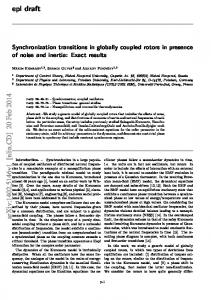
FIG. 1: (color online) Synchronization diagrams r(λ) for different networks constructed using the interpolation model introduced in [25]. The α values in each panel are (a) α = 1 (ER), (b) α = 0.6, (c) α = 0.2 and (d) α = 0 (BA). The four panels show both Forward and Backward continuations in λ using increments of δλ = 0.02. The size of the networks is N = 103 and the average degree is hki = 6.
is the distribution of the natural frequencies, {ωi }, and it is assumed to be unimodal and even [23]. Here we will focus on the influence of the dynamical and topological characteristics at the local level (the nodes of the network and their interactions) in the emergence of global synchronization. In particular, we will identify the internal frequency of each node i directly with its degree ki , so that ωi = ki in Eqs. (1). Note that this prescription automatically sets that the distribution of frequencies g(ω) = P (k) but not vice versa [24]. To study the effects of the correlation between dynamical and structural attributes, we simulate the Kuramoto model on top of a family of networks generated according to [25]. This model allows to construct networks with the same average connectivity, hki, interpolating from Erd¨os-R`enyi (ER) graphs to Barab`asi-Albert (BA) SF networks by tuning a single parameter α. The growth of the networks assumes that a newly added node either attaches randomly with probability α or preferentially to those nodes with large degree with probability (1 − α). In this way, α = 1 gives rise to ER graphs with a Poissonian degree distribution whereas for α = 0 the resulting networks are SF with P (k) ∼ k −3 . Intermediate values α ∈ (0, 1) tune the heterogeneity of the network, which increases when going from α = 1 to α = 0. In the four panels of Fig. 1, we report the synchronization diagrams of four network topologies constructed using this model. The limiting cases of ER and BA networks correspond to panel 1a and 1d, respectively. The size of these networks are N = 103 while the average connectivity is set to hki = 6. For each panel in Fig. 1 we have computed two synchronization diagrams, r(λ), labeled as Forward and Backward continuations. The former diagram is computed by increas-
ing progressively the value of λ and computing the stationary value of the order parameter r for λ0 , λ0 + δλ,..., λ0 + nδλ. Alternatively, the backward continuation is performed by decreasing the values of λ from λ0 + nδλ to λ0 . The panels 1a, 1b and 1c show a typical second-order transition with a perfect match between the backward and forward synchronization diagrams. Importantly, the onset of synchronization is delayed as the heterogeneity of the underlying graph (and thus that of the frequency distribution g(ω)) increases. The most striking result is however observed for the BA network (panel 1d) in which a sharp, first-order synchronization transition appears. In the case of the forward continuation diagram the order parameter remains r ≃ 0 until the onset of synchronization in which r jumps suddenly to r ≃ 1 pointing out that almost all the network has reached the synchronous motion. Moreover, the diagram corresponding to the backward continuation also shows a sharp transition from the fully synchronized state to the incoherent one. The two sharp transitions takes place at different values of r so that the whole synchronization diagram displays a strong hysteresis. To analyze deeply the change of the order of the synchronization transition, we have monitored the evolution of the dynamics for every node by computing their effective frequency along the forward continuation, see Fig. 2 . The effective frequency of a node i is defined as Z 1 t+T ˙ eff θi (τ ) dτ , (3) ωi = T t with T ≫ 1. We have also computed the evolution of ωieff within a degree class k, hωik , averaging over nodes having identical degree k: 1 X eff ωi , (4) hωik = Nk [i|ki =k]
where Nk = N P (k) is the number of nodes with degree k in the network. From the panels in Fig. 2 we observe that the individual frequencies and the different curves hωik (λ) converge progressively to the average frequency of the system Ω = hki = 6 until full synchronization is achieved. Panel 2a (ER graph) shows that the convergence to Ω is first achieved by those nodes with large degree while the small k-classes achieve full synchronization later on. As the heterogeneity of the network increases (see α = 0.6 and α = 0.2 in panels 2b and 2c, respectively) the differences in the convergence of the k-classes decrease. Finally, for the BA network (Fig. 2d), we observe that nodes (and thus the different k-classes) retain their natural frequencies until they become almost fully locked, which signal the abrupt synchronization observed in Fig. 1d. Thus, the first-order transition of the BA network corresponds to a process in which no microscopic signals of synchronization are observed until the critical coupling λc is reached. To further explore the correspondence of the explosive synchronization transition with the SF nature of the underlying graph, in Fig. 3.a we show the synchronization diagrams for
3 1
1
0.8
0.8
γ=3.3 γ=3.0 γ=2.7 γ=2.4
0.6
r
0.6
γ=3.3 γ=3.0 γ=2.7 γ=2.4
r
0.4
0.4
0.2
0.2
(a)
(b)
0
0 1
1.5
2
2.5
3
3.5
0
0.5
1
1.5
λ
2
2.5
3
3.5
λ
FIG. 3: (color online) Panel (a) shows the synchronization diagrams r(λ) for several SF networks constructed via the configurational model. All the networks have a degree-distribution P (k) ∼ k−γ with γ = 2.4, 2.7, 3.0, and 3.3 while N = 103 . The steps of the continuation are set to δλ = 0.02. In panel (b) we show the synchronization diagrams of the same SF networks without the local correlation between degrees and natural frequencies, i.e. ωi 6= ki , while the distribution of natural frequencies is still P (ω) ∼ ω −γ . FIG. 2: (color online) The panels show the evolution of the effective frequencies of the nodes along the (forward) continuation in the four model networks of Fig. 1. The colored dots account for single-node values (colors stand for their respective degree) while the solid lines show the evolution of the average value of the effective frequencies of nodes having the same degree.
different uncorrelated SF graphs with different degree distribution’ exponents. These graphs have been constructed using the configurational model [26] by imposing a degree distribution P (k) ∼ k −γ with γ = 2.4, 2.7, 3.0 and 3.3. The synchronization diagrams are obtained by forward continuation (as described above) starting at λ = 1 and performing adiabatic increments of δλ = 0.02. Again, for each value of λ the Kuramoto dynamics is run until the value of r reaches its stationary state. From the figure it is clear that a first-order synchronization transition appears for all the reported values of γ pointing out the ubiquity of the explosive synchronization transition in SF networks. Moreover, the onset of synchronization, λc , is delayed as γ decreases, i.e. when the heterogeneity of the graph increases. Up to now, we have shown that the explosive synchronization transition appears in SF when the natural frequencies of the nodes are correlated with their degrees. To show that this correlation is the responsible of such explosive transition, in Fig. 3b we show the synchronization diagram for the same SF networks used in Fig. 3a, but when the correlation between dynamics and structure is broken in such a way that the same distribution for the internal frequencies, g(ω) = ω −γ is kept. To this end, we made a random assignment of frequencies to nodes according to g(ω). The plots reveal that now all the transitions turn to be of second-order, thus recovering the usual picture of synchronization phenomena in complex networks. Therefore, the first-order transition arises due to the positive correlation between natural frequencies and the degrees of the nodes in SF networks [27]. All the simulations results presented corroborate our conjecture about the explosive percolation transition in SF networks. To get analytical insights, we reduce the problem stud-
ied to the analysis of the star configuration, a special structure that grasp the main property of SF networks, namely the role of hubs. Therefore, we explore the synchronization transition of such a configuration and show that it is indeed explosive when the correlation ωi = ki holds. A star graph (as shown in the inset of Fig. 4a) is composed by a central node (the hub) and K peripheral nodes (or leaves). Each of the peripheral nodes connects solely to the hub. Thus, the connectivity of the leaves is ki = 1 (i = 1, ..., K) while that of the hub is kh = K. Let us suppose that the hub has a frequency ωh while all the leaves beat at the same frequency ω. First we set a reference frame rotating with the average phase of the system, Ψ(t) = Ψ(0) + Ωt, being Ω the average frequency of the oscillators in the star, Ω = (Kω + ωh )/(K + 1). In the following we set Ψ(0) = 0 without loss of generality so that the transformed variables are defined as φh = θh −Ωt for the hub and φj = θj −Ωt (with j = 1, ..., K) for the leaves. Thus, the equations of motion for the hub and the leaves read: φ˙h = (ωh − Ω) + λ
K X
sin(φj − φh ),
(5)
j=1
φ˙j = (ω − Ω) + λ sin(φh − φj ), with j = 1...K.(6) In this rotating frame the motion of the hub, Eq. (5), can be expressed as: φ˙h = (ωh − Ω) + λ(K + 1)r sin(φh ) ,
(7)
note that in this new frame it is easy to identify that the dynamics of the hub is governed by its new inherent frequency and the superposition of a set of identical signals from the leaves. Now, imposing that the phase of the hub is locked, φ˙h = 0, we obtain: sin φh =
(ωh − Ω) . λ(K + 1)r
(8)
4 1
1
0.8
K=10
0.8 0.6
0.6
of the distribution of natural frequencies. Our findings provide with an explosive phase transition of an important macroscopic phenomena, synchronization, in a widely studied dynamical framework, the Kuramoto model, thus shedding light to the microscopic roots behind these phenomena and paving the way to their study in other dynamical contexts.
K=20 K=30 K=40 K=50 K=60 K=70
K (K+1)
r
r
0.4
0.4
0.2
0.2 0 0.5 (K−1) 1.1 (K+1)
Backward Forward
1.4
1.7 λ
2
2.3
0 2.6
2
2.5
3
3.5
4 λ
4.5
5
5.5
6
FIG. 4: (color online) We show the synchronization diagrams for the star graph [see the inset in plot (a)]. In (a) we show the (forward and backward) continuation diagrams for the case K = 10 while (b) shows the forward continuation diagrams for different star graphs of different sizes, corresponding to K = 20, 30, 40, 50, 60 and 70.
Now we consider the equations for the leaves, Eq. (6), and evaluate the expression for cos φj in the locked regime, φ˙ j = 0. After some algebra, we obtain the following expression: q� � (Ω − ω) sin φh ± 1 − sin2 φh [λ2 − (Ω − ω)2 ] cos φj = . λ (9) The above expression is valid only when (Ω − ω) ≤ λ. From this inequality we obtain the value of the coupling λ for which the phase-locking is lost, i.e. the critical coupling λc = Ω−ω. In our case, we have ωh = K, ω = 1 and Ω = 2K/(K + 1) so that we obtain a critical coupling λc = (K − 1)/(K + 1). On the other hand, we can derive the value rc of the order parameter at the critical point by using Eq. (8) and Eq. (9) to compute r = hcos(φ)i at λc : K cos(φh ) + K cos(φj ) . (10) = rc = K +1 (K + 1) λc Therefore, as rc > 0, when the synchronization is lost there is a gap in the synchronization diagram pointing out the existence of a first-order synchronization transition. Moreover, as K increases both λc and rc tend to 1 thus confirming the first-order nature of the transition in the thermodynamic limit, K → ∞. As shown in Fig. 4a for the case K = 10, the theoretical values of λc and rc , are in perfect agreement with results from numerical simulations. Finally, as shown in Fig. 4b, the stability of the unlocked phase regime, r ≃ 0, increases with K so that we can reach larger values of λ by continuing (forward) the solution with r ≃ 0. As a result, this robustness of the incoherent solution leads to a larger hysteresis cycle of the synchronization diagram as K increases. Summing up, we have shown that an explosive synchronization transition occurs in SF networks when there is a positive correlation between the structural (the degrees) and dynamical (natural frequencies) properties of the nodes. This constitutes the first example of an explosive synchronization transition in complex networks. Moreover, we have shown that the emergence of such transition is intrinsically due to the interplay between the local structure and the internal dynamics of nodes rather than being caused by any particular form
J.G.-G. is supported by the MICINN through the Ram´on y Cajal Program. This work has been partially supported by the Spanish DGICYT Grants FIS2008-01240, MTM200913848, FIS2009-13364-C02-01, FIS2009-13730-C02-02, and the Generalitat de Catalunya 2009-SGR-838.
[1] A.T. Winfree, The geometry of biological time (SpringerVerlag, New York, 1990). [2] S.H. Strogatz, Sync: The Emerging Science of Spontaneous Order (New York: Hyperion, 2003). [3] A. Pikovsky, M. Rosenblum and J. Kurths, Synchronization: a universal concept in nonlinear sciences (Cambridge University Press, 2003). [4] D.J. Watts and S.H. Strogatz, Nature 393, 440-442 (1998). [5] S.H. Strogatz, Nature 410, 268-276 (2001). [6] S. Boccaletti et al., Phys. Rep. 424, 175-308 (2006). [7] A. Arenas et al., Phys. Rep. 469, 93 (2008). [8] Y. Moreno and A.F. Pacheco, EPL 68, 603-609, (2004). [9] D.-S. Lee, Phys. Rev. E 72, 026208 (2005). [10] A. Arenas, A. D´ıaz-Guilera and C.J. Perez-Vicente, Phys. Rev. Lett. 96, 114102, (2006). [11] C. Zhou and J. Kurths, Chaos 16, 015104 (2006). [12] J. G´omez-Garde˜nes, Y. Moreno and A. Arenas, Phys. Rev. Lett. 98, 034101 (2007). [13] L.M. Pecora and T.L. Carroll, Phys. Rev. Lett. 80, 2109-2012 (1998). [14] M. Barahona and L.M. Pecora, Phys. Rev. Lett. 89, 054101 (2002). [15] T. Nishikawa et al., Phys. Rev. Lett. 91, 014101 (2003). [16] C. Zhou, A.E. Motter and J, Kurths, Phys. Rev. Lett. 96, 034101 (2006). [17] D. Achlioptas, R.M. D’Souza, and J. Spencer, Science 323, 1453 (2009). [18] F. Radicchi and S. Fortunato, Phys. Rev. Lett. 103, 168701 (2009). [19] Y.S. Cho et al., Phys. Rev. Lett. 103, 135702 (2009). [20] Y. Kuramoto, Lect. Notes in Physics 30, 420-422 (1975). [21] Y. Kuramoto, Chemical oscillations, waves, and turbulence (Springer-Verlag, New York, 1984). [22] J.A. Acebron et al., Rev. Mod. Phys. 77, 137-185 (2005). [23] S. H. Strogatz, Physica D 143, 1 (2000). [24] It is worth stressing that our main results hold when wi ∼ kiα with α > 0, i.e. when wi is positively correlated with ki . [25] J. G´omez-Garde˜nes and Y. Moreno, Phys. Rev. E 73, 056124 (2006). [26] M. Molloy and B. Reed, Rand. Struct. Alg. 6, 161 (1995). [27] We have also measured the synchronization diagrams for different cases of intermediate degree-frequency correlation. To this end, we initially assign ωi = ki with probability (1 − p) while, with probability p, ωi is randomly drawn from a distribution P (ω) ∼ ω −γ . In the supplementary figure 5 we show the diagrams r(λ) for different values of p in a SF network with γ = 2.4. It is shown that for p > 0 explosive synchronization
5 remains while at some value pc < 1 the transition turns into a second-order one.
6
1
p=0.1 p=0.3 p=0.5 p=0.7 p=0.9
0.8
r
0.6 0.4 0.2 0 0
0.5
1
1.5
2 λ
2.5
3
3.5
4
FIG. 5: Synchronization diagrams for intermediate degree-frequency correlation (see [27] for further details).


![Synchronization in Microwave Networks [PDF]](https://m.moam.info/img/260x300/synchronization-in-microwave-networks-pdf_64963fbb098a9eb61a8b4593.jpg)