Extending a Resolution Prover for Inequalities on Elementary Functions

Extending a Resolution Prover for Inequalities on Elementary Functions Behzad Akbarpour and Lawrence C. Paulson Computer Laboratory, University of Cambridge, England {ba265,lcp}@cl.cam.ac.uk

Abstract. Experiments show that many inequalities involving exponentials and logarithms can be proved automatically by combining a resolution theorem prover with a decision procedure for the theory of real closed fields (RCF). The method should be applicable to any functions for which polynomial upper and lower bounds are known. Most bounds only hold for specific argument ranges, but resolution can automatically perform the necessary case analyses. The system consists of a superposition prover (Metis) combined with John Harrison’s RCF solver and a small amount of code to simplify literals with respect to the RCF theory.

1

Introduction

Despite the enormous progress that has been made in the development of decision procedures, many important problems are not decidable. In previous work [1], we have sketched ideas for solving inequalities over the elementary functions, such as exponentials, logarithms, sines and cosines. Our approach involves reducing them to inequalities in the theory of real closed fields (RCF), which is decidable. We argued that merely replacing occurrences of elementary functions by polynomial upper or lower bounds sufficed in many cases. However, we offered no implementation. In the present paper, we demonstrate that the method can be implemented by combining an RCF decision procedure with a resolution theorem prover. The alternative approach would be to build a bespoke theorem prover that called theory-specific code. Examples include Analytica [8] and Weierstrass [6], both of which have achieved impressive results. However, building a new system from scratch will require more effort than building on existing technology. Moreover, the outcome might well be worse. For example, despite the well-known limitations of the sequent calculus, both Analytica and Weierstrass rely on it for logical reasoning. Also, it is difficult for other researchers to learn from and build upon a bespoke system. In contrast, Verifun [10] introduced the idea of combining existing SAT solvers with existing decision procedures; other researchers grasped the general concept and now SMT (SAT Modulo Theories) has become a well-known system architecture. Our work is related to SPASS+T [17], which combines the resolution theorem prover SPASS with a number of SMT tools. However, there are some differences

between the two approaches. SPASS+T extends the resolution’s test for unsatisfiability by allowing the SMT solver to declare the clauses inconsistent, and its objective is to improve the handling of quantification in SMT problems. We augment the resolution calculus to simplify clauses with respect to a theory, and our objective is to solve problems in this theory. Our work can therefore be seen to address two separate questions. – Can inequalities over the elementary functions be solved effectively? – Can a modified resolution calculus serve as the basis for reasoning in a highly specialized theory? At present we only have a small body of evidence, but the answer to both questions appears to be yes. The combination of resolution with a decision procedure for RCF can prove many theorems where the necessary case analyses and other reasoning steps are found automatically. An advantage of this approach is that further knowledge about the problem domain can be added declaratively (as axioms) rather than procedurally (as code). We achieve a principled integration of two technologies by using one (RCF) in the simplification phase of the other (resolution). We eventually intend to output proofs where at least the main steps are justified. Claims would then not have to be taken on trust, and such a system could be integrated with an interactive prover such as Isabelle [16]. The tools we have combined are both designed for precisely such an integration [13, 15]. Paper outline. We begin (§2) by presenting the background for this work, including specific upper and lower bounds for the logarithm and exponential functions. We then describe our methods (§3): which axioms we used and how we modified the automatic prover. We work through a particular example (§4), indicating how our combined resolution/RCF solver proves it. We present a table of results (§5) and finally give brief conclusions (§6).

2

Background

The initial stimulus for our project was Avigad’s formalization, using Isabelle, of the Prime Number Theorem [2]. This theorem concerns the logarithm function, and Avigad found that many obvious properties of logarithms were tedious and time-consuming to prove. We expect that proofs involving other so-called elementary functions, such as exponentials, sines and cosines, would be equally difficult. Avigad, along with Friedman, made an extensive investigation [3] into new ideas for combining decision procedures over the reals. Their approach provides insights into how mathematicians think. They outline the leading decision procedures and point out how easily they perform needless work. They present the example of proving 1 + y2 1 + x2 < (2 + y)17 (2 + x)10 from the assumption 0 < x < y: the argument is obvious by monotonicity, while mechanical procedures are likely to expand out the exponents. To preclude this

possibility, Avigad and Friedman have formalized theories of the real numbers in which the distributivity axioms are restricted to multiplication by constants. As computer scientists, we do not see how this sort of theory could lead to practical tools or be applied to the particular problem of logarithms. We prefer to use existing technology, augmented with search and proof heuristics to this problem domain. We have no interest in completeness—these problems tend to be undecidable anyway—and do not require the generated proofs to be elegant. Our previous paper [1] presented families of upper and lower bounds for the exponential and logarithm functions. These families, indexed by natural numbers, converge to their target functions. The examples described below use some members of these families which are fairly loose bounds, but adequate for many problems.

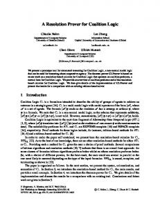
3x2 − 4x + 1 x−1 ≤ ln x ≤ x 2x2

“1 2

” ≤x≤1

2

−x + 4x − 3 ≤ ln x ≤ x − 1 2

(1 ≤ x ≤ 2)

−x2 + 8x − 8 x ≤ ln x ≤ 8 2

(2 ≤ x ≤ 4)

Fig. 1. Upper and Lower Bounds for Logarithms

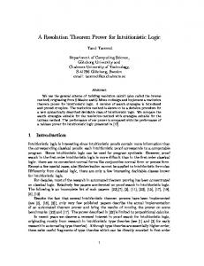
x3 + 3x2 + 6x + 6 x2 + 2x + 2 ≤ exp x ≤ 6 2 2 6 ≤ exp x ≤ x2 − 2x + 2 −x3 + 3x2 − 6x + 6

(−1 ≤ x ≤ 0) (0 ≤ x ≤ 1)

Fig. 2. Upper and Lower Bounds for Exponentials

Figure 1 presents the upper and lower bounds for logarithms used in this paper. Note that each of these bounds constrains the argument to a closed interval. This particular family of bounds is only useful for finite intervals, and proofs involving unbounded intervals must refer to other properties of logarithms, such as monotonicity. Figure 2 presents upper and lower bounds for exponentials, which are again constrained to narrow intervals. Such constraints are necessary: obviously there exists no polynomial upper bound for exp x for unbounded x, and a bound like ln x ≤ x − 1 is probably too loose to be useful for large x. Tighter constraints on the argument allow tighter bounds, but at the cost of requiring case analysis on x, which complicates proofs. Our approach to proving inequalities is to replace occurrences of functions such as ln by suitable bounds, and then to prove the resulting algebraic inequal-

ity. Our previous paper walked through a proof of −

1 ≤ x ≤ 3 =⇒ ln(1 + x) ≤ x. 2

(1)

One of the cases reduced to the following problem:  2 x 1 −x ≤x + 1+x 2 1+x As our paper shows, this problem is still non-trivial, but fortunately it belongs to a decidable theory. We have relied on two readable histories of this subject [9, 15]. Tarski proved the decidability of the theory of Real Closed Fields (RCF) in the 1930s: quantifiers can be eliminated from any inequality over the reals involving only the operations of addition, subtraction and multiplication. It is inefficient: the most sophisticated decision procedure, cylindrical algebraic decomposition (CAD), can be doubly exponential. We use a simpler procedure, implemented by McLaughlin and Harrison [15], who in their turn credit H¨ormander [12] and others. For the RCF problems that we generate, the decision procedure usually returns quickly: as Table 1 shows, most inequalities are proved in less than one second, and each proof involves a dozen or more RCF calls. Although quantifier elimination is hyper-exponential, the critical parameters are the degrees of the polynomials and the number of variables in the formula. The length of the formula appears to be unimportant. At present, all of our problems involve one variable, but the simplest way to eliminate quotients and roots involves introducing new variables. We do encounter situations where RCF does not return. Our idea of replacing function occurrences by upper or lower bounds involves numerous complications. In particular, most bounds are only valid for limited argument ranges, so proofs typically require case splits to cover the full range of possible inputs. For example, three separate upper bounds are required to prove equation (1). Another criticism is that bounds alone cannot prove the trivial theorem 0 < x ≤ y =⇒ ln x ≤ ln y, which follows by the monotonicity of the function ln. Special properties such as monotonicity must somehow be built into the algorithm. Search will be necessary, since some proof attempts will fail. If functions are nested, the approach has to be applied recursively. We could have written code to perform all of these tasks, but it seems natural to see whether we can add an RCF solver to an existing theorem prover instead. For the automatic theorem prover, we chose Metis [13], developed by Joe Hurd. It is a clean, straightforward implementation of the superposition calculus [4]. Metis, though not well known, is ideal at this stage in our research. It is natural to start with a simple prover, especially considering that the RCF decision procedure is more likely to cause difficulties.

3

Method

Most resolution theorem provers implement some variant of the inference loop described by McCune and Wos [14]. There are two sets of clauses, Active and Passive. The Active set enjoys the invariant that every one of its elements has been resolved with every other, while the Passive set consists of clauses waiting to be processed. At each iteration, these steps take place: – An element of the Passive set (called the given clause) is selected and moved to the Active set. – The given clause is resolved with every member of the Active set. – Newly inferred clauses are first simplified, for example by rewriting, then added to the Passive set. (They can also simplify the Active and Passive sets by subsumption, an important point but not relevant to this paper.) Resolution uses purely syntactical unification: no theory unification is involved. Our integration involves modifying the simplification phase to take account of the RCF theory. Algebraic terms are simplified and put into a canonical form. Literals are deleted if the RCF solver finds them to be inconsistent with algebraic facts present in the clauses. Both simplifications are essential. The canonical form eliminates a huge amount of redundant representations, for example the n! permutations of the terms of x1 +· · ·+xn . Literal deletion generates the empty clause if a new clause is inconsistent with existing algebraic facts, and more generally it eliminates much redundancy from clauses. To summarize, we propose the following combination method: 1. Negate the problem and Skolemize it, finally converting the result into conjunctive normal form (CNF) represented by a list of conjecture clauses. 2. Combine the conjecture clauses with a set of axioms and make a problem file in TPTP format, for input to the resolution prover. 3. Apply the resolution procedure to the clauses. Simplify new clauses as described below before adding them to the Passive set. 4. If a contradiction is reached, we have refuted the negated formula. 3.1

Polynomial Simplification

All terms built up using constants, negation, addition, subtraction, and multiplication can be considered as multivariate polynomials. Following Gr´egoire and Mahboubi [11], we have chosen a canonical form for them: Horner normal form, also called the recursive representation.1 An alternative is the distributed representation, a flat sum with an ordering of the monomials; however, our approach is often adopted and is easy to implement. Any univariate polynomial can be rewritten in recursive form as p(x) = an xn + · · · + a1 x + a0 = a0 + x(a1 + x(a2 + · · · x(an−1 + xan )) 1

A representation is called canonical if two different representations always correspond to two different objects.

We can consider a multivariate polynomial as a polynomial in one variable whose coefficients are themselves a canonical polynomial in the remaining variables. We maintain a list with the innermost variable at the head, and this will determine the arrangement of variables in the canonical form. We adopt a sparse representation: zero terms are omitted. For example, if variables from the inside out are x, y and z, then we represent the polynomial 3xy 2 + 2x2 yz + zx + 3yz as [y(z3)] + x([z1 + y(y3)] + x[y(z2)]), where the terms in square brackets are considered as coefficients. Note that we have added numeric literals to Metis: the constant named 3, for example, denotes that number, and 3 + 2 simplifies to 5. We define arithmetic operations on canonical polynomials, subject to a fixed variable ordering. For addition, our task is to add c + xp and d + yq. If x and y are different, one or other is recursively added to the constant coefficient of the other. Otherwise, we just compute (c + xp) + (d + xq) = (c + d) + x(p + q), returning simply c + d if p + q = 0. For negation, we recursively negate the coefficients, while subtraction is an easy combination of addition and negation. We can base a recursive definition of polynomial multiplication on the following equation, solving the simpler sub-problems p × d and p × q recursively: p × (d + yq) = (p × d) + (0 + y(p × q)) However, for 0 + y(p × q) to be in canonical form we need y to be the topmost variable overall, with p having no variables strictly earlier in the list. Hence, we first check which polynomial has the earlier topmost variable and exchange the operands if necessary. Powers pn (for fixed n) are just repeated multiplication. Any algebraic term can now be translated into canonical form by transforming constants and variables, then recursively applying the appropriate canonical form operations. We simplify a formula of the form X ≤ Y by converting X − Y to canonical form, finally generating an equivalent form X 0 ≤ Y 0 with X 0 and Y 0 both canonical polynomials with their coefficients all positive. We simplify 1 + x ≤ 4 to x ≤ 3, for example. Any fixed format can harm completeness, but note that the literal deletion strategy described below is indifferent to the particular representation of a formula. 3.2

Literal Deletion

We can distinguish a literal L in a clause by writing the clause as A ∨ L ∨ B, where A and B are disjunctions of zero or more literals. Now if ¬A ∧ ¬B ∧ L is inconsistent, then the clause is equivalent to A ∨ B; therefore, L can be deleted. We take the formula ¬A ∧ ¬B ∧ L to be inconsistent if the RCF solver reduces it to false. For example, consider the clause x ≤ 3 ∨ x = 3. (Such redundancies arise frequently.) We focus on the first literal and note that x 6= 3 ∧ x ≤ 3 is consistent, so that literal is preserved. We focus on the second literal and note that

¬(x ≤ 3) ∧ x = 3 is inconsistent, so that literal is deleted: we simplify the clause to x ≤ 3. This example illustrates a subtle point concerning variables and quantifiers. In the clause x ≤ 3 ∨ x = 3, the symbol x is a constant, typically a Skolem constant originating in a existentially quantified variable in the negated conjecture. Before calling RCF, we again convert x to an existentially quantified variable. Here is a precise justification of this practice. In the semantics of firstorder logic [5], a structure for a first-order language L comprises a non-empty domain D and interprets the constant, function and relation symbols of L as corresponding elements, functions and relations over D. The clause x ≤ 3 ∨ x = 3 is satisfied by any structure that gives its symbols their usual meanings over the real numbers and also maps x to 3; it is, however, falsified if the structure instead maps x to 4. To prove the inconsistency of say ¬(x ≤ 3) ∧ x = 3, we give the RCF solver a closed formula, ∃x [¬(x ≤ 3) ∧ x = 3]; if this formula is equivalent to false, then there exists no interpretation of x satisfying the original formula. More generally, we can prove the inconsistency of a ground formula by existentially quantifying over its uninterpreted constants before calling RCF. We strengthen this test by taking account of all algebraic facts known to the prover. (At present, we consider only algebraic facts that are ground.) Whenever the automatic prover asserts new clauses, we extract those that concern only addition, subtraction and multiplication. We thus accumulate a list of algebraic clauses that we include in the formula that is delivered to the RCF solver. For example, consider proving − 21 ≤ u ≤ 3 =⇒ ln(u + 1) ≤ u. Upon termination, it has produced the following list of algebraic clauses: F, ~(1