Nov 23, 2005 - Train classifier with respect to the weighted sample set {S, d(t)} and obtain ..... in Neural Information Processing Systems, David S. Touretzky,.
Face Detection with Mixtures of Boosted Discriminant Features Julien Meynet, Vlad popovici and Jean-Philippe Thiran Ecole Polytechnique F´ed´erale de Lausanne (EPFL) Signal Processing Institute CH-1015 Lausanne, Switzerland.
Technical report TR-ITS-2005.35 November 23, 2005
Abstract Detecting faces in images is a key step in numerous computer vision applications as face recognition for example. Face detection is a difficult task in image analysis because of the large face intra-class variability which is due to the important influence of the environmental conditions on the face aspect. The existing methods for face detection can be divided into holistic methods and feature based methods. We propose a new method for detecting frontal faces in complex images featuring two main contributions: the use of a collection of highly discriminative anisotropic Gaussian features combined by boosting and the computation using a mixture of classifiers to improve the classification capabilities without affecting the detection speed. The performances of the face detector have been evaluated on the CMU/MIT test set [1] database. This methods outperforms the previous works in frontal face detection.
keywords: face detection, AdaBoost, Gaussian features, mixtures of classifiers
1
Introduction
Automatic face detection is a key step in any face processing system. Its goal is to detect the presence of human faces in a still image and return their position (which may be given in terms of a bounding box for example). The performance of latter stages of processing (e.g. face recognition, face authentication or facial expression recognition) is conditionned by the quality of the detection. However automatic detection of faces is far from being an immediate task. Its complexity is due to the large intra-class variability, as faces are highly deformable objects whose appearance depends on numerous factors (lighting conditions, presence or absence of occluding objects, and so forth). In most face detection system, it is necessary to model also the ”non f ace” class, which proves to be very difficult. In the last years, many methods have been proposed and we give hereafter a brief overview of some of the most significant ones. There are two main approaches for detecting faces: Holistic methods which consider the face as a global object and feature based methods which use classical low level processing for detecting faces (e.g. skin color modeling). Other technique can also use a mix of both appoaches. The first category usualy produce a very fast detector 1
Meynet J. TR-ITS-2005.35
2
with better classification performances and they turn out to be more robust to light changes. One of the main advantages of the feature-based methods is that they are more robust to head pose changes. As we are interested in further face processing such that face recognition, we only need to detect frontal faces, that is why in the following, only the holistic methods will be considered. More detailed surveys are given in [2] and [3]. In general, the image is scanned with a sliding window and for each position, the window is classified as either face or non face. The method can be applied at different scales (and possibly different orientations) for detecting faces of various sizes. Finally, after the whole search space has been explored, an arbitration technique may be employed for eliminating the multiple detections. Of course the efficient exploration of the search space is a key ingredient for obtaining a fast face detector. There are various methods for speeding up this search, like using additional information (e.g. skin color) or using a coarse-to-fine approach. Nevertheless the most important component of the system is the classifier deciding if a given window contains a face or not. From this perspective, this paper focuses on both aspects, efficient search space and robust classifier. A first reference algorithm is proposed by Sung and Poggio [4]. They use clusters of face and non face models to decide if a constant sized window contains a face or not. The principle is to use several gaussian clusters to model both the face and non face examples in the vector space. Then the decision is taken according to the relative distance to both classes. In order to detect faces at any scale and position they use a sliding window which scans a pyramid of images. A similar holistic approach proposed by Rowley et. al. in [5] is one of the most representative for the class of neural network approaches. It comprises two modules: a classification module which hypothesizes the presence of a face and a module for arbitrating multiple detections. A fast algorithm is proposed by Viola and Jones in [6]. It is based on three main ideas. They first train a strong classifier by boosting the performance of simple rectangular Haarlike features. They use the so-called integral image as image representation which allows to compute the base classifiers very efficiently. Finally they introduce a classification structure in cascade in order to improve both the detection speed and the classification results. This last method (in particular the cascade structure) leads to a very fast detection (about 25 frames per second on a conventional PC). As it will be explained later in the paper, we have used this method as a pre-processing step in order to reduce the search space. In this work we present a new approach which uses two main components. First we introduce anisotropic Gaussian discriminative local features (GF) combined by boosting and then a mixture of parallel classifiers which are combined using probability rules to output the final decision. The local features that are proposed in this paper present the advantage of being more discriminative than the Haar-like features introduced in [6]. It turns out that they are particularly well suited for the representation of face images. On the other hand the mixture of classifier reduces the complexity of the training process while improving the classification performances. This idea of splitting a complex problem into several lower complexity problems has been discused in [7] and [8], where the combination of a number of locally trained Support Vector Machiness (SVM) is done either by a linear SVM or using some other combination rules. A review of how classifiers can be combined together can be found in [9]. Figure 1 shows an overview of the complete face detection system. The remaining of the paper is structured as follows. Section 2 introduces the new geometrical features and discusses their ability to model the face patterns. It also gives a brief overview of AdaBoost, a learning algorithm that selects iteratively the best of these features. Section 3 presents the mixtures of boosted classifiers and how they are combined together to perform
Meynet J. TR-ITS-2005.35
3
Scanned input image
Cascade of Haar features stage 1 stage 2
stage N
Mixtures of Gabor features
Mix 1
Mix 2
Mix M
Combination rule
Figure 1: Overview of the face detection system. the final decision. Section 4 reports some results as well as comparisons with relevant existing face detectors. Finally, we draw some conclusions and explain the future work in section 5.
2 2.1
Boosted anisotropic Gaussian features AdaBoost
Training a statistical face detector consists in learning a model from a set of face and non face patterns. This section explains how we build this model using a learning algorithm called AdaBoost. From the input images we extract a collection of local features which, associated with thresholds, form a collection of very simple linear classifiers called weak classifiers. Then a strong classifier is obtained by linear combination of some of these weak classifiers. The coefficients of the linear combination as well as the features themselves are trained using a boosting algorithm called AdaBoost [10] (for Adaptive Boosting). It combines iteratively the weak classifiers by taking into account a weight distribution on the training samples. The algorithm is described in Algorithm (2.1). The basic idea is to focus on the examples that are misclassified at the current iteration. AdaBoost was proposed in 1995 by Freund and Shapire [10] as an efficient algorithm of the ensemble learning field. It is a greedy algorithm which constructs an additive combination of weak classifiers such that it minimizes the exponential loss defined in Eq (1). L(y, f (x)) = exp(−yf (x)),
(1)
Meynet J. TR-ITS-2005.35
4
Algorithm 2.1: Discrete AdaBoost algorithm[10] 1
Input: S = (x1 , y1 ), . . . , (xN , yN ), Number of iterations T
2
Initialize: dn = 1/N for all n = 1, . . . , N for t = 1, . . . , T, do
3
(1)
1. Train classifier with respect to the weighted sample set {S, d(t) } and obtain hypothesis ht : x 7→ {−1, +1}, i.e. ht = L(S, d(t) ) 2. Calculate the weighted training error ²t of ht : ²t =
N X
d(t) n I(ym 6= ht (xn )),
n=1
3. Set: αt =
1 1 − ²t , log 2 ²t
4. Update the weights: (t)
dn exp(−αt yn ht (xn )) , Zt P (t+1) =1. where Zt is a normalization constant such that N n=1 dn d(t+1) = n
4 5
end Break if: ²t = 0 or ²t ≤ 12 and set T = t − 1 P Output: fT (x) = Tt=1 PTαt ht (x) r=1
αt
where x if the pattern to be classified, y its target label and f (x) the decision function. One of the interests of this iterative algorithm is that the training error converges exponentially towards zero and in practice the generalization error continues decreasing with the number of iteration when the null training error is reached. Freund and al. in [10] showed that the generalization error is bounded by: Ãr ! d R[fT ] ≤ P [yfT (x) ≤ θ] + O , ∀θ > 0, (2) N θ2 where fT is the decision function output by AdaBoost, d is the VC-dimension defined by Vapnik in [11] and N is the number of examples. This bound in Eq. (2) is quite loose but it shows that larger margins lead to smaller upper bound on the testing error. Like many other learning algorithms, AdaBoost has an important drawback. It tends to overfit training samples when they are noisy. The influence of the noisy samples will be discussed in section 3. Note that we usually prefer detecting all the faces and accept more false alarms than taking an equal error rate. We can thus build an asymmetric version of AdaBoost by encouraging the correct classification of the positive examples. This can be done for example by penalizing the negative examples in the initial sample weight distribution. The final threshold is also tuned on an independent validation set in order to obtain the desired operating point on the ROC curve.
Meynet J. TR-ITS-2005.35
2.2
5
Anisotropic Gaussian features
In this section we describe the visual local features that are used to construct the weak classifiers. They are constructed from base functions of an overcomplete basis. It means that the expansion of any image in this base is not unique. These features have been recently used in image compression and signal approximation fields. They were first introduced by Peotta and al. in [12]. The generative function φ(x, y) : R2 → R is described in Eq. (3) 2
φ(x, y) = xe−(|x|+y ) .
(3)
It is made of a combination of a Gaussian and its first derivative. This presents the ability of approximating efficiently contour singularities with a smooth low resolution function in the direction of the contour and it approximates the edge transition in the orthogonal direction. Different transformations can be applied to this generative function: 1. Translation by (x0 , y0 ): Tx0 ,y0 φ(x, y) = φ(x − x0 , y − y0 ). 2. Rotation by θ: Rθ φ(x, y) = φ(x cos θ − y sin θ, x sin θ + y sin θ). 3. Bending by r: ½ Br φ(x, y) =
p y φ(r − (x − r)2 + y 2 , r arctan( r−x )) if x < r φ(r − |y|, x − r + r π2 ) if x ≥ r
4. Anisotropic scaling by (sx , sy ): Ssx ,sy φ(x, y) = φ(
x y , ). sx sy
By combining these four basic transformations, we obtain a large collection of ψsx ,sy ,θ,r,x0 ,y0 functions as defined in Eq. (4) and (5). Denote D this collection.
ψi (x, y) = ψsx ,sy ,θ,r,x0 ,y0 (x, y) = Tx0 ,y0 Rθ Br Ssx ,sy φ(x, y).
(4) (5)
Figure 2 shows some of these atoms with various bending and rotating parameters. Now we want to construct a classifier based on these geometrical features that best separate the face and non face classes. The first step is thus to construct a simple linear classifier with each atom configuration by choosing two classifier parameters, a threshold θj and a parity pj as shown in Eq. (6). Parameters θj and pj are chosen using Bayes decision rule. ½ hj (x) =
1 if pj fj (x) < pj θj , 0 otherwise
(6)
Meynet J. TR-ITS-2005.35
6
Figure 2: Anisotropic Gaussian features with different rotating and bending parameters. where fj (x) is the inner product between the image and the base function number j, ψj corresponding to a particular parameter configuration (sx , sy , θ, r, x0 , y0 ) (see Eq. (7)). ZZ ∀ψi ∈ D
fi (x) =
X×Y
ψi (x, y)I(x, y) dxdy.
(7)
Of course each of these classifiers is not discriminant enough to be used alone as a robust face detector. It is what we call a base classifier (or weak classifier in the boosting terminology in the sense that each of these simple classifier only has to classify better than the random selection) as introduced in Section 2.1.
2.3
Gaussian vs. Haar-like
This section shows a comparison between the Haar-like features (HF) proposed in [6] and the anisotropic Gaussian features (GF) described above. A very important advantage of the HF is that they can be computed extremely efficiently using a so called integral image representation. The HF are made of 2, 3 or 4 rectangular masks with 2 scaling parameters and two center coordinates. The templates are shown in Figure 1. These simple features are in fact simple combinations of discretised versions of very particular GF with no bending and only orthogonal rotations. Moreover, HF are only binary features such that they may be able to well capture the contrast between image regions but it will be intuitively limited for differentiating faces and complicated non face images (face-like images) as for example high textured images. GF are continuous functions more likely to model continuous natural images. The parameter flexibility allows to model contour singularities as well as intensity changes in large regions (with large scaling parameters). We now give numerical comparisons between HF and GF. Two boosted classifiers have been trained on the same training set containing face and non face images using the simple Discrete AdaBoost algorithm described in algorithm (2.1). The results are evaluated on a large test set. Figure 3 gives a comparison of the intrinsic performances of each feature type. The test error decreases quickly with the number of Adaboost iterations but it stops decreasing after roughly 100 iterations in the case of HF while it continues decreasing for with GF. Intuitively, after several iterations, AdaBoost focuses on the hard to classify examples and the simplistic Haar features are not discriminant enough to separates the two classes. The better performances of the Gaussian features also clearly appears in the ROC analysis (Figure 4)( The Receiver Operating Characteristic (ROC) curves are drawn by changing the threshold output by AdaBoost). An intersting point to notice here is the shape of the GF that are selected by AdaBoost. The
Meynet J. TR-ITS-2005.35
7
15 Gabor Haar 14
13
Test error rate (%)
12
11
10
9
8
7
6
5
0
50
100
150
200
250
300
350
400
450
No selected features
Figure 3: Gaussian vs. Haar-like evaluation on a test set. first features selected have generally large scale parameters, they can globally model the face appearance whereas more local features are extracted later in the selection process. Let us now evaluate the time needed for computing each feature. We trained two similar classifiers with 200 HF on the first hand and 200 GF on the second hand. By appling these two classifiers on several images (without any structure in cascade), we compared the average computation time for applying a single HF and a single GF. Computing a GF takes roughly 2.86 more time than a HF. (Note that the Gaussian features are precomputed in the model such that the expensive generative function computation is avoided). As mentionned before, a sliding window is used to scan the whole image. In fact scanning an image requires testing a huge number of windows. In this set of windows, only few of them contain a face and a large majority of them are very easy to discard. In this case it is useless to apply a complex classifier in the complete image. Moreover, as it appears in the first iterations in Figure 3, Haar-like features are comparatively efficient for building the first linear classifiers. In order to use their computation efficiency (especially if they are built in a cascade structure), a simple five staged cascade of Haar-like features has been added as a pre-processing to our Gaussian-based classifier. This efficiently reduces the search space.
3 3.1
Mixtures of boosted classifiers Motivations
The combination of weak geometrical features is itself a good classifier but this section introduces a structure that will improve the classifications skills of the face detection system. As already mentionned in the introduction, the complexity of face detection resides in the fact that a very large set of faces and non-face examples must be collected. Moreover a really huge number of features is needed to obtain a sufficiently low false positive rate. AdaBoost minimizes an exponential loss function (see Eq. (1)) so that after several iterations, many
Meynet J. TR-ITS-2005.35
8
100
True positive rate (%)
95
90
85
80
Gabor Haar 75
0
5
10
15
20
25
False positive rate (%)
Figure 4: ROC curves for Gaussian and Haar-like features. features have to be added for slightly reducing the false positive rate. On the other hand, some variation in the face training examples is needed in order to be able to detect faces with slight pose variations and with slight scale changes (taking into account the scaling factor). A large training dataset is necessary to cover all this variability. Because of this large number of samples needed to train the models, some weak classifiers potentially very efficient on local subspaces of the data may behave badly with respect to the whole training set. These motivations suggest to use a multi-classifier structure built in parallel. Instead of training a single boosted classifier on the complete training set, we built several classifiers on subsets of the original dataset. A similar technique was developed and discussed in [7] where Support Vector Machines were used for the parallel classifiers. There are many interesting points in such an approach. On the first hand, each mixture is trained on a local subset of the classes distributions so that it focuses on its own domain. It will thus decrease the influence of potential outliers in the complete training set. More specifically, as the power of AdaBoost resides in the fact that it focuses on the hard to classify examples, the parallelization technique reduces the weight of the noisy examples or potential outliers. This last point also reduces the risk of overfitting as mentionned above. From a practical point of view it will decrease the false positive rate which is a important in the face detection context. On the second hand it keeps an equivalent training complexity. The complexity of training AdaBoost varies linearly with the number of samples. Splitting the data and training several AdaBoosted classifiers on the subsets will thus not affect the training complexity compared to a single AdaBoosted classifier. We could imagine two strategies for splitting the dataset into several subsets. Either random sampling if we want to estimate several times the decision boundary or clustering if we want to build experts on subsets of the face class. In our case, no information is available about the distribution of the face class, we just want to simplify the problem while improving the classification skills, that is why simple random sampling has been chosen for creating
Meynet J. TR-ITS-2005.35
9
the subsets. Another reason why the clustering would not be appropriate comes from the variations introduced in the training set. The clustering would eventually cluster examples resulting from similar transformations of the initial images and thus the combination would probably fail.
3.2
Posterior probability estimation
Once the multiple classifiers have been built the final decision is taken using classical probability rules. In this step we need a probabilistic interpretation for each boosted classifier and then arbitrating using typical rules such as maximum, minimum, product, sum, median or majority vote. First recall that AdaBoost minimizes the exponential criterion: J(f ) = E(e−yf (x) ).
(8)
Friedman in [13] shows that minimizing J(f ) in Eq. (8) is equivalent up to second order Taylor expansion about f = 0 to maximizing the expected binomial log-likelihood. The posterior probabilities P (y = 1|x) and P (y = −1|x) are given by the following lemma:
Lemma 3.1 [13] J(f ) = E(e−yf (x) ) is minimized at f (x) =
1 P (y = 1|x) log . 2 P (y = −1|x)
Hence P (y = 1|x) =
(9)
ef (x) , e−f (x) + ef (x)
(10)
e−f (x) e−f (x) + ef (x)
(11)
P (y = −1|x) =
Several different strategies may be used for combining parallel classifiers. An overview of them can be found in [9] and [14]. In this work we only consider the summation rule defined in Eq. (12) for combining the decisions of the multiple boosted classifiers. This means that example x is assigned to the class y = 1 (face) if: (1 − M )P (y = 1) +
X
Pj (y = 1|x) >
j=1,..,M
(1 − M )P (y = −1) + 1
X j=1,..,M
Pj (y = −1|x) (12)
Meynet J. TR-ITS-2005.35
10
where M is the number of mixtures and p(y = 1), p(y = −1) represents the prior probabilities for both classes. Otherwise, x is assigned to the class y = −1 (non face). The choice of this rule is influenced by the splitting method that is used. The sum rule averages the decisions of the individual classifiers so that it is good trade off for discarding false alarms while preserving the correct detection of faces. For example the product rule is known to be a severe rule which risks to strongly penalize the true positive rate. More comments about the choice of the decision criterion are given in [9]. A reason why simple probability rules are used for combining the expertise of each individual classifier is the stability of the parallel classifiers. The boosted classifiers are stable in the sense that small changes in the training set lead to small changes in the classifier output [14]. Bagging or Boosting for combining base classifiers needs unstable classifiers to improve the overall performance.
3.3
Discussion
This parallelization technique presents some advantages against the cascade structure. A cascade of classifiers is a sequential combination of classifiers such that an example is rejected if it is classified as negative at any stage of the cascade. It is equivalent to a parallel structure of classifiers but considering a product probability rule for combining the decisions. In fact if we consider the parallel classifiers to be conditionally independent (which can be supposed in this study as we use random sampling for generating the subsets), if one of the classifiers considers an example as negative with probability close to 1, the probability that the final decision is negative will be high. The only difference would be from the complexity point of view as we would have to test all the classifiers whereas the cascade would directly stop the processing chain. One advantage of our parallel approach over the cascade is that if a positive example is classified as negative by a given classifier, it can be reassigned to the positive class by the overall system where in the cascade case it would be rejected. This would especially happen in the last stages of the cascade as the examples becomes more and more complicated. It is clear that the mixture approach will not reduce the testing time as we roughly use the same features number as in a single layer classifier. However we do not need to optimize the testing time as we only need to test a few remaining critical windows.
4 4.1
Experiments and results Structure of the system
In order to test the performances of this system and compare it with other relevant methods the following experiments have been performed. First of all the input image is scanned with a cascade of 5 boosted Haar-like stages (according to Viola’s methods in [6]). This discards very quickly the easy to classify non face windows. In the scanning process, we use a scaling factor of 1.2 for resizing the sliding window. All the remaining windows are resized at 20 × 15 pixels and given to the mixture of boosted classifiers which takes the final decision. Then a very simple arbitration method clusters the neighbor windows in order to only have one detection per face. This is done by keeping the median window for each cluster.
Meynet J. TR-ITS-2005.35
11
Figure 5: Results on images of BANCA [18] in the complex adverse scenario. First of all, face images were collected from some classical face databases: XM2VTS [15], BioID [16], FERET [17]. After adding some variations in scale and slight rotations and shifts, the complete face train set contained 9500 images. The non faces examples were chosen by bootstrapping on randomly selected images without faces and pre-processed by the Haar cascade. In our model we used 5 parallel mixtures each of them trained with 1900 faces and 4000 non face images. Each mixture is made of roughly 200 features, which corresponds to desired true positive rate / false positive rate ratio on a validation set. Note that the set of HF that we used to train the preprocessing model contained 37520 (all possible combinations in a 20 × 15 pixels window. In the case of the GF, we decided to sample randomly the dictionary order to keep a managable set for the training process. We finally used a dictionary of 202200 features.
4.2
BANCA database
The system has been tested on two distinct databases. On the first hand we consider the BANCA database [18] which was build for training and testing multi-modal verification systems. The face images were acquired using various cameras and under several scenarios (controlled, degraded and adverse). Some examples of detection results of the adverse scenario are shown in Figure 5. For four different languages, images of 52 persons (26 males and 26 females) were recorded during 12 sessions. We finally only used the French and English databases as we dispose of precise groundtruth annotations for them. An ambiguous point in face detections algorithms is the way the performances are measured. The criterion used to evaluate face detectors on labeled dataset may be confusing. Different works use different criteria to consider a detection as correct or wrong. It becomes very difficult to compare objectively different algorithms. This problem is addressed using the evaluation protocol proposed by Popovici and al. in [19]. The evaluation is performed by taking into account several parameters between the detected location and the annotated positions. The scoring function measures the ratio of the betweeneyes distances, the angle between the eyes axis and of course the distance between the annotated and detected eye positions. This method gives a more objective scoring of the detection performances. See [19] for details on how to use the scoring function. Table 1 gives a comparison of three variants that have been tested on the BANCA database which represents 12480 images, each of them containing one face. It shows several interesting points. First of all we see that a single boosted Gaussian features (BGF) classifier stage (pre-
Meynet J. TR-ITS-2005.35
12
Table 1: Comparisons of 3 tested methods on the BANCA [18] database. Results are reported for the French and English parts following the evaluation protocol described in [19]. Detections with a global score larger than 95% are considered as correct. Classifier English(%) French(%) Total (%) 5 stages BHF 48.08 56.09 52.08 12 st. BHF 73.64 94.26 83.95 5 st. BHF + 1 st. BGF 80.79 93.94 87.36 5 st. BHF + Mix of BGF 95.21 97.53 96.37 Table 2: Performances on the CMU/MIT test set [1]. It shows the Detection rate (D.R.) and number of false alarms (F.A) for each method. Set B (483) (507) Methods D.R. F.A. D.R. F.A. D.R. F.A. Rowley [5] 87.1 15 92.5 862 90.5 570 Sung Poggio [4] 81.9 13 — — — — Shneiderman [20] — — 93.0 88 94.4 65 Viola Jones [6] — — — — 91.4 50 Mixture of BGF 89.2 15 92.1 68 93.9 60 processed by 5 HF stages) outperforms a 12 stages boosted Haar-like features (BHF) system. It confirms the choice of the GF. This is also emphazised by the fact that less selected features are needed for achieving better classification performances. It means that the sparsest model (BGF) produces a better generalization than BHF. Then the mixture improvements clearly appear in these results. The single Gaussian stage was trained using the same data than the complete mixture and roughly the same number of atoms were selected for both cases however the mixtures performs better. The evaluation protocol [19] allows us to measure the main characteristics of our detector. Each individual criterion in Figure 6 shows that the wrong detections are generally far from the ground truth position but when a detection is correct, it is really precise both in scale and shift (and of course also in angle as we only test upright faces). However, there is a slight imprecision with respect to the shift score. This can be explained by the trivial arbitration criterion that we use for clustering the multiple detections around each face.
4.3
CMU/MIT Test set
We now consider a more challenging database comonly used to evaluate performances of face detectors especially on very low resolution images. The CMU/MIT Test set [1] was first introduced by Rowley in [5] for testing. It contains 130 images with 507 faces. Some of these annotated faces are manually drawn and they are counted as false detections in some papers. That is why some papers only consider 123 images with 483 faces. Both versions are tested in this paper to avoid any confusion. Finally TestSet B contains 23 images with a total of 155 faces. Figure 8 shows some detection results on images of this database. Table 2 presents comparisons with the state-of-the-art methods on this databases. In order to give a complete comparison study, we tested the system on several configurations of the test
Meynet J. TR-ITS-2005.35
13
Figure 6: Detection scores using the evaluation protocol [19] including the two individual scores (shift and scale) and the global score. Note that a log scale is used. ROC for CMU/MIT Test Set 100 Rowley Shneiderman Viola Mix BGF
True positive rate (%)
95
90
85
80
75
70
0
100
200
300
400
500
600
# False Alarms
Figure 7: ROC analysis for comparing the algorithms on the MIT/CMU testset [1].
Meynet J. TR-ITS-2005.35
14
set as presented in other studies. The manually drawn faces that are detected in the setup with 507 faces are counted as false detections in the setup with only 483 faces. It explains why there are more false detections in the smallest version of the test set. Finally, in order to give more comprehensive results, we give a complete Receiver Operating Characteristic curve (ROC). Notice that we give the detection rate as function of the number of false negative instead of false positive rate as this last one highly depends on the scanning operator. It can be seen that the proposed approach outperforms the other methods for these real world low resolution images. The detector of Shneiderman and al. [20] gives a better operating point. However their technique is based on a complex network which is very slow (roughly 1 minute to test an image) and is difficult to use in real applications.
Figure 8: Face detection results on some images of the MIT/CMU testset [1].
Meynet J. TR-ITS-2005.35
5
15
Conclusions
This paper presents a new face detection system using a multi-stage feature based approach which leads to high detection performances and can be applied in real-time. Two main contributions are presented. On the first hand, new local discriminant features are combined by boosting to model efficiently the face class. On the second hand several parallel boosted classifiers are combined in order to build a strong classifier. It has been shown how the new features improve the haar-like features and also that the mixture of boosted classifiers decreases significantly the false positive rate without affecting the true positive rate. The complete system has been tested on classical databases and compared with other relevant methods. In a future work we will pay more attention on the combination of the parallel classifiers and especially study the influence of mixtures dependences on the combination behavior.
Acknowledgments This work is supported by the Swiss National Science Foundation through the National Center of Competence in Research on ”Interactive Multimodal Information Management (IM2)”.
References [1] Henry A. Rowley, Shumeet Baluja, and Takeo Kanade, “Neural network-based face detection,” IEEE Transactions on Pattern Analysis and Machine Intelligence, vol. 20, no. 1, pp. 23–38, 1998. [2] Erik Hjelmas and Boon Kee Low, “Face detection: a survey,” In Computer Vision and Image Understanding [2], pp. 236–274. [3] M. Yang, D. Kriegman, and N. Ahuja, “Detecting faces in images: a survey,” In IEEE transactions on Pattern Analysis and Machine Intelligence [3]. [4] Kah Kay Sung and Tomaso Poggio, “Example-based learning for view-based human face detection,” IEEE Transactions on Pattern Analysis and Machine Intelligence, vol. 20, no. 1, pp. 39–51, 1998. [5] Henry A. Rowley, Shumeet Baluja, and Takeo Kanade, “Human face detection in visual scenes,” in Advances in Neural Information Processing Systems, David S. Touretzky, Michael C. Mozer, and Michael E. Hasselmo, Eds. 1996, vol. 8, pp. 875–881, The MIT Press. [6] Paul Viola and Michael J. Jones, “Robust real-time face detection,” Int. J. Comput. Vision, vol. 57, no. 2, pp. 137–154, 2004. [7] Julien Meynet, Vlad Popovici, and Jean-Philippe Thiran, “Face class modeling using mixture of svms,” in In Proceedings of International Conference on Image Analysis and recognition, ICIAR 2004, Porto, Portugal, J. Bigun, Ed., Berlin, September 2004, EPFL, Springer-Verlag. [8] Julien Meynet, Vlad Popovici, and Jean-Philippe Thiran, “Combining svms for face class modeling,” in 13th European Signal Processing Conference - EUSIPCO, 2005.
Meynet J. TR-ITS-2005.35
16
[9] Josef Kittler, Mohamad Hatef, Robert P. W. Duin, and Jiri Matas, “On combining classifiers,” IEEE Trans. Pattern Anal. Mach. Intell., vol. 20, no. 3, pp. 226–239, 1998. [10] Yoav Freund and Robert E. Schapire, “A decision-theoretic generalization of on-line learning and an application to boosting,” J. Comput. Syst. Sci., vol. 55, no. 1, pp. 119–139, 1997. [11] Vladimir N. Vapnik, The nature of statistical learning theory, Springer-Verlag New York, Inc., New York, NY, USA, 1995. [12] L. Peotta, L. Granai, and P. Vandergheynst, “Very low bit rate image coding using redundant dictionaries,” in Proceedings of the SPIE, Wavelets: Applications in Signal and Image Processing X. SPIE, November 2003, vol. 5207, pp. 228–239, SPIE. [13] Jerome Friedman, Trevor Hastie, and Robert Tibshirani, “Additive logistic regression: A statistical view of boosting,” The Annals of Statistics, vol. 28, pp. 337–407, 2000. [14] Ludmila I. Kuncheva, Combining Pattern Classifiers Methods and Algorithms, John Wiley, New York,, New York, NY, USA, 2004. [15] K Messer, J Matas, J Kittler, J Luettin, and G Maitre, “Xm2vtsdb: The extended m2vts database,” in Second International Conference on Audio and Video-based Biometric Person Authentication, March 1999. [16] Robert W. Frischholz and Ulrich Dieckmann, “Bioid: A multimodal biometric identification system,” Computer, vol. 33, no. 2, pp. 64–68, 2000. [17] P.J. Phillips and al., “The FERET database and evaluation procedure for facerecognition algorithms,” in Image and Vision Computing, March 1999, vol. 16. [18] E. Bailly-Bailliere and al., “The banca database and evaluation protocol,” in 4th International Conference on Audio- and Video-Based Biometric Person Authentication, Guildford, UK, Berlin, June 2003, vol. 2688 of Lecture Notes in Computer Science, pp. 625–638, Springer-Verlag. [19] V. Popovici, J. Thiran, Y. Rodriguez, and S. Marcel, “On performance evaluation of face detection and localization algorithms,” in Proceedings of the 17th International Conference on Pattern Recognition, J. Kittler, Ed. August 2004, vol. 1, pp. 313–317, IEEE. [20] H. Schneiderman and T. Kanade, “A statistical approach to 3d object detection applied to faces and cars,” in International Conference on Computer Vision, 2000.