Constraint merging tableaux maintain a system of all closing substitutions of ..... The function calls mergeBuf which performs the actual work. Its first two param-.
Fair Constraint Merging Tableaux in Lazy Functional Programming Style Reiner H¨ ahnle and Niklas S¨ orensson Chalmers University of Technology & G¨ oteborg University Department of Computing Science S-41296 Gothenburg, Sweden {reiner,nik}@cs.chalmers.se
Abstract. Constraint merging tableaux maintain a system of all closing substitutions of all subtableau up to a certain depth, which is incrementally increased. This avoids backtracking as necessary in destructive first order free variable tableaux. The first sound and complete implementation of this paradigm was given in an object-oriented style by Giese. In this paper we analyse the reasons why lazy functional implementations so far were problematic (although appealing), and we give a solution. The resulting implementation in Haskell is compact and modular. The input language includes far-reaching control and extension mechanisms.
1
Introduction
Until recently, implementations of free variable tableau proof procedures suffered from the necessity to backtrack over branch closing substitutions, if completeness was not to be sacrificed [9]. The central problem is that substitutions destructively change the rigid variables occurring in tableaux, which leads to complex dependencies between substitution and extension steps. Then, almost simultaneously, two different ways to solve this problem popped up: both, Baumgartner et al. [2, 3] and Beckert [4, 5] found ways to “repair” a tableau after a destructive closure step. The details of both approaches are rather different, but they have in common that the resulting proof procedures have unusual and relatively complicated rules. Perhaps this is the reason why a serious implementation of these ideas was not tried so far. A fundamentally different way to cope with destructive closing substitutions is to simply enumerate all possible closing substitutions of a tableau in parallel. The fact that substitutions can be seen as term constraints suggests the phrase constraint tableaux [10] for a tableau procedure along these lines. Traditionally, this has been considered as too expensive in order to be viable and, if one uses naive breadth-first search, it certainly is. The breakthrough came with Giese’s work [6–8] who suggested to associate a “lazy” stream of closing substitutions associated with the subtableau below each tableau node. This requires to merge streams of closing sustitutions to be merged, so the resulting calculi are called constraint merging tableaux. In combination with further refinements, such as
pruning, subsumption, and simplification, it is on the way to becoming a competitive implementation [8]. Giese’s implementation is object-oriented and realized in Java, but the term “lazy” suggests to use a programming language supporting lazy evaluation. Such implementations in the lazy functional language Haskell were given by Van Ei´ Nuall´ jck [11, 12] and O ain [10]. Our approach is related to the latter. Both, however, suffer from certain drawbacks, which we try to remedy in this paper. A lazy functional implementation is less straightforward than it seems at first. At the heart of such a constraint tableau implementation is the merging of streams of substitutions at branching nodes. If refute yields a stream of closing substitutions for a set of formulas, then the code for disjunctive formulas looks like this: refute {φ ∨ ψ} ∪ B = merge (refute {φ} ∪ B) (refute {ψ} ∪ B) The merger drives lazy evaluation of subtableaux. As we show below, one must design it very carefully to ensure fairness (and, hence, completeness). This was not properly addressed in functional implementations so far. Another problem is that any competitive implementation of a tableau-based proof procedure needs to incorporate refinements such as pruning and subsumption. Giese [8, p 45] reports that an attempt to combine fairness and refinements in a functional style resulted in a merger of overwhelming complexity. Van Eijck’s [11, 12] and ´ Nuall´ O ain’s [10] implementations are not fair (as we show below) and do not feature efficiency refinements. In this paper we present a constraint merging tableaux procedure in lazy functional style. Specifically, we make the following contributions: (a) we clearly identify and describe the fairness problems present in previous approaches (Section 2.4) and we show how they can be cleanly solved (Section 2.5); (b) we demonstrate that a comparatively elegant, almost “lean” (less than 100 lines, we give almost the full code), and complete implementation in lazy functional style is possible (Section 2.3); (c) in our input formula language one can include arbitrary Haskell functions, which we show to have certain advantages (Section 2.1, 2.2); (d) we describe some refinements we implemented towards a competitive incarnation of the procedure (Section 3). The source code is available at http://www.cs.chalmers.se/~nik/lazy.
2
The implementation
In Van Eijck’s implementation [11, 12], explicit data structures are built up to ´ Nuall´ represent tableaux, while O ain [10] dispenses with that and keeps only the system of term constraints that would result from applying the rules. Universally quantified formulas are handled by so-called seeds, which are constraints that can duplicate themselves with fresh variables. In our approach the notion of a formula is central. To be more precise, we exploit that certain kinds of first order formulas completely determine a tableaux for them up to the substitutions applied. A formula is identified with a Haskell function that produces a stream of closing substitutions for this formula and a given tableau branch.
2.1
Terms and Formulas
Expressions of type TT (for tableau template) are potentially infinite tableaux corresponding to a first order formula. The interface of type TT is as follows: fresh :: (Term -> TT) -> TT pLit :: Atom -> TT nLit :: Atom -> TT
() :: TT -> TT -> TT () :: TT -> TT -> TT
The types Atom and Term that occur in it, are defined below; think of them as abstract representations of terms and atoms. The functions of TT can be seen as formula constructors (in Haskell syntax): pLit and nLit allow to build positive and negative literals, respectively; and can be used to construct disjunctive and conjunctive formulas, respectively. For example, the formula φ = (¬p ∨ q) ∧ ¬q could be constructed as follows: phi = (nLit p pLit q) nLit q
(1)
Like in Skolemized Negation Normal Form (SNNF), we only allow disjunction, conjunction, plus negation at the literal level. Universal quantification is a bit more complicated and will be discussed below. Here is the representation of first order terms: data Term = Var VarId | Fun String [Term] type Atom = Term It allows to declare signatures in an intuitive way by lifting first order functions (and predicates) to Haskell functions. Functions have a string identifier, while variables are identified by a unique label generated by the system. For simplicity, atoms are typed as terms. The following code declares a constant zero, a oneplace function suc, and a one-place predicate nat (the latter is distinguished from functions only by its usage). zero = Fun "zero" [] suc x = Fun "suc" [x] nat x = Fun "nat" [x] Now we can build formulas containing variables. Consider, for example, the definition: sucNat x = nLit (nat x) pLit (nat (suc x)) Here, we view the formula sucNat(x) with free variable x as a Haskell function sucNat with formal parameter x. As a welcome consequence, substitution can be realized simply as function application. For example, evaluation of “sucNat t” yields the formula, in which each occurrence of x is replaced by t. At the heart of first order theorem proving is the capability to obtain unlimited numbers of fresh instances of universally quantified formulas. We provide
directly an operation called fresh that takes a formula with a free variable and produces an instance, where the free variable has been replaced with a new unique (ie, “fresh”) name. It is important to understand the difference between a formula with a free variable and a fresh instance of it: the former is realized as a Haskell function from variables to formulas, an example being sucNat above. The operator fresh takes as its parameter such a function from variables to formulas and replaces in it each variable occurrence with a fresh name (how this is done in a functional style will be explained later). For example, we can write fresh sucNat to obtain a fresh instance of sucNat (with respect to x), say: sucNat’ = nLit (nat x’) pLit (nat (suc x’)). The formula resulting from an application of fresh does, of course, no longer depend on x. The new name that x was replaced with (in sucNat’ it is x’) is later used as a (rigid) free variable in the tableau sense, that is, it is mapped to at most one substitution term. But x’ in sucNat’ will never be syntactically replaced henceforth. In the following, when we write “parameter”, we mean a function parameter in the sense of the programming language Haskell. When we write “free variable” we mean it in the sense of tableau proofs. To obtain the universal closure of sucNat (with respect to x), we take an “operational” view of the universal quantifier realized by Haskell’s recursion mechanism: uSucNat = fresh sucNat uSucNat. In this way we obtain an infinite supply of fresh instances of sucNat as the expression is evaluated. Strict evaluation of the expression defining uSucNat does not terminate, but Haskell’s lazy evaluation semantics prevents this. We can view it as a (finite) representation of the infinite term “fresh sucNat fresh sucNat ...”. 1 As we will see (in Fig. 3), the implementation of conjunction is sensitive to the order of its parameters: the definition “uSucNat = uSucNat fresh sucNat”, for example, would not terminate.
2.2
Tableau Representation
The correspondence between recursive definitions and infinite terms suggests a reading of expressions with type TT as certain tableaux. Formally, let us call a free variable tableau for a formula φ, to which no closure rule has been applied, a tableau template. Note that a tableau template, in general, is an infinite tree. To illustrate this, we extend the uSucNat example, which uses universal formulas as explained in the previous section. 1
´ Nuall´ This approach somewhat resembles O ain’s seeds [10].
zeroIsNat twoIsNotNat sucNat x uSucNat countToTwo
= = = = =
pLit (nat zero) nLit (nat (suc (suc zero))) nLit (nat x) pLit (nat (suc x)) fresh sucNat uSucNat zeroIsNat twoIsNotNat uSucNat
This corresponds to the following first order formula: nat(0) ∧ ¬nat(s(s(0))) ∧ (∀ x)(¬nat(x) ∨ nat(s(x)))
(2)
But in fact the tableau building functions of type TT do much more than representing a formula: they build the tableau template displayed in Fig. 1. nat(0) ¬nat(s(s(0))) ¬nat(x0 ) ¬nat(x1 ) .. .
nat(s(x1 )) .. .
nat(s(x0 )) ¬nat(x2 ) .. .
nat(s(x2 )) .. .
Fig. 1. Infinite tableau corresponding to a recursive formula definition.
The tableau in Fig. 1 is just one of infinitely many possible tableaux that can be constructed for formula (2), however, it is completely determined by the particular definition we gave for countToTwo. We happened to arrange the constituents of countToTwo in a fair manner, hence, tableau completeness guarantees that the tableau in Fig. 1 can be completed to a proof. It is not possible to specify any • • admissible tableau for a given formula ¬p q ¬q with the help of the Haskell tableau building operations. Nonetheless, we ¬q ¬q q ¬p are able to exercise a great deal more control than is usually possible with Fig. 2. Tableau templates for different the input to a theorem prover. Be- formula orders. fore explaining how tableau building works, let us examplify the flexibility of our approach. The tableau corresponding to the code in (1) is displayed in on the very left. Specifying the same formula with differently ordered constituents, e.g. nLit q (pLit q nLit p), results in a different tableau (displayed on the right). Next we illustrate how the formula input language can be mixed with arbitrary Haskell code to make it more expressive. Let us define a little function that produces n conjoined copies of a formula f:
nTimes 1 f = f nTimes n f = f nTimes (n-1) f With its help it is easy to realize a resource-bounded quantifier that allows to use at most n instances of its scope. A small change to the previous example suffices: uSucNat x = nTimes n (fresh sucNat) The effect here is that the tableau in Fig. 1 is cut off after the (n + 2)-nd level. In particular, we are allowed to use n instances of sucNat on each branch. Our example problem “counts” to 2. Via Haskell it is easy to make it parametric to count up to an arbitary number. First, define count 0 = zero count n = suc (count (n-1)) This can be used to define natural numbers in the “natural” way: nIsNotNat n = nLit (nat (count n)) A tableau like the one depicted in Fig. 1 with n + 2 levels can “count” to 2n−1 + 1 (the maximal number of instances of sucNat occurring in it). Using both bounded quantification and the parametric formulation it is, therefore, possible to prove the following problem (where we use some mathematical typography to ease reading): logSucNat n = nTimes (dlog2 n − 1e+1) (fresh sucNat) countNat n = zeroIsNat nIsNotNat n logSucNat n We conclude this subsection with the slightly surprising demonstration that the language of tableau templates allows even to control the shape of proofs. The following definition, for example, forces tableaux for the counting example to become linear: linSucNat x = nLit (nat x) (pLit (nat (suc x)) fresh linSucNat) countNat n = zeroIsNat nIsNotNat n fresh linSucNat The trick is that recursion is only done in the right part of the disjunction, which leads to linear trees. We should also mention that one drawback of our notation is that universal quantification cannot be directly expressed, but we have to go through an explicit recursion. On the other hand, it is possible to automatically translate every SNNF formula into an equivalent formula in our language. 2.3
Tableau Construction
In this section we explain in detail how the tableau template operators are implemented. Let us first get a technicality out of the way.
Fresh Variable Names Recall that the fresh operator is used to create copies of formulas, where free variables are renamed to unique labels that are guaranteed not to occur elsewhere in the tableau. Since the implementation is functional, we cannot use a global counter mechanism to create fresh variables, and since tableau templates are potentially infinite structures, it is not possible to give a monadic formulation (otherwise the “standard” solution in Haskell for situations like this). Therefore, we need to pass a variable generator through all operators. It is not necessary to understand its implementation details. Just keep in mind that in the following the formal parameter vg denotes a variable generator. Think of vg as an infinite set of variable identifiers from which we are able to choose one that has not been used so far. It is possible to create a new variable generator with the operation newVG. 2 The crucial point is that a variable generator (that is, an infinite set of names) can be split with splitVG into two generators that do not overlap. This is used in the tableau branching operator. To obtain a new variable from a generator vg one uses “takeVG vg”. This yields a pair (v,nvg) whose first component is a so far unused variable v, and whose second component is a new generator nvg that “knows” that v cannot be used any longer. Substitutions and Unification There is a type Subst that represents substitutions. The only thing one needs to know about them is that one can perform unification and intersection: unify :: Term -> Term -> Maybe Subst intersect :: Subst -> Subst -> Maybe Subst Intersection is intended to compute the conjunction of its parameters when seen as constraints on terms. The data type Maybe gives the standard extension of a given type by an error element (called Nothing in Haskell). This is required, because two given terms may not be unifiable and two term constraints may be incompatible. Tableau Templates A branch is a simple record datatype that contains fields for a variable generator and two lists of atoms (for the positive, respectively, the negative literals on the branch): data Branch = Br VGen [Atom] [Atom] type TTC = Branch -> Stream Subst type TT = TTC -> TTC The functions of type TTC (for tableau template continuation) are supposed to take a branch and give a stream of all possible closing substitutions for this branch. For technical reasons (explained in Sections 2.4, 2.5 below), in reality it is necessary to use doubly nested lists of substitutions as the result type. To enhance readability, we hide these behind a simple abstract type called Stream 2
This operation is actually an IO action in our implementation. This allows us to have a non pure, but efficient, implementation of the variable generator.
with obvious conversion functions toList, toStream as well as concatenation (the precise definitions are given in Section 2.5). The actual interface for tableau templates is defined on a separate (but isomorphic) type TT in order to make it possible to define operators in “continuation passing style”. We use TTC for a closed tableau (yet to be computed) and TT for a tableau with “holes”. We illustrate this when discussing the TT operators below. Tableau Template Implementation Now we have everything together to describe the core of our theorem prover: the implementation of the operators on tableau templates. The top level function is: runTT :: TT -> IO [Subst] runTT tt = do vg toStream []) (Br vg [] []) ) ) First we explain the type of runTT: it expects a tableau template (for example, “countNat 3” as defined in Section 2.2) and yields a list of closing substitutions for it.3 The result type is an IO operation, merely because newVG is one. Now to the implementation of runTT: first, an initial variable generator vg is provided and used to construct an initial branch (Br vg [] []) without any atoms. The tableau template parameter tt has type TTC -> TTC. Recall that TTC declares a function from branches to streams. The purpose is to properly terminate the whole construction. It is merely required if the tableau is going to contain a finite branch, in which case we need to terminate the streams with [] saying “no more substitutions”. The result of applying tt to this terminating continuation again has type TTC. It expects a branch—the initial branch—and goes on to produce the list of closing substitutions. To understand how this is done, we need to look into the implementation of the constructors used in TT as listed in Section 2.1. pLit :: Atom -> TT pLit a c b = toStream (closeP a b) c (extendP a b) nLit :: Atom -> TT nLit a c b = toStream (closeN a b) c (extendN a b) The typing of the literal constructors is not obvious. Expansion of the type of pLit and nLit yields: TTC }| { z Atom -> TTC -> Branch | {z -> Stream} TT By currying, this is equivalent to a function mapping a triple of an atom a, a continuation c, and a branch b to streams. 3
In general, this list of closing substitutions is infinite. In most cases, one would wrap a prove function around runTT, which aborts the computation after the first substitution arrives.
The idea for functions nLit and pLit is first to compute all closing substitutions of the literal a with the current branch b. Then compute the closing substitutions when the current branch, extended with a, is given to continuation c. Finally, concatenate both streams. Here are the auxiliary functions used above: extendP, extendN :: Atom -> Branch -> Branch extendP a (Br vg pos neg) = Br vg (a:pos) neg extendN a (Br vg pos neg) = Br vg pos (a:neg) closeP, closeN :: Atom -> Branch -> [Subst] closeP a (Br _ _ neg) = mapMaybe (unify a) neg closeN a (Br _ pos _) = mapMaybe (unify a) pos Both extendP and extendN are obvious. The function mapMaybe used in closeP, closeN is like a standard map function, but filters out those applications that yielded Nothing. Next we describe the the fresh operation: fresh :: (Term -> TT) -> TT fresh f c (Br vg pos neg) = let (v,nvg) = takeVG vg in f v c (Br nvg pos neg) The typing can be explained similarly as for nLit and pLit above: the function fresh has the current continuation c and the current branch (Br vg pos neg) as second and third parameter. The first parameter is now a function from variables to formulas and represents the formula, of which we want a fresh instance. First we obtain a fresh name v and a new variable generator nvg as explained above. Instantiation can be realized by simply applying the function f to v. To the result we pass the current continuation and a suitably updated (with nvg) branch. To realize sequential conjunction, we simply use function composition, denoted by the symbol “.” in Haskell: () :: TT -> TT -> TT () tx ty = tx . ty The effect of the operation is to plug the tableau template ty into the open branches of the tableau template tx as illustrated in Fig. 3.
tx
ty
tx
⇒ ty
...
ty
Fig. 3. Illustration of sequential conjunction of tableau templates.
The disjunction operator is implemented, at least on the abstract level, relatively straightforwardly. Its typing again can be explained similarly as for nLit and pLit above. () :: TT -> TT -> TT () tx ty c (Br vg pos neg) = let (l,r) = splitVG vg (lb, rb) = (Br l pos neg, Br r pos neg) in merge (tx c lb) (ty c rb) The main point is to split the variable generator so that different variables are being used for renaming. Then the streams of both subtableaux are merged. The tricky part is the merging, and we devote the rest of this section to it. First we explain, why merging is difficult, then we present our solution. 2.4
The Difficulty of Merging Substitutions
1. nat(zero) 2. -nat(suc(suc(zero)))
3. -nat(X2) X2=zero@1 4. -nat(X3) X3=zero@1
5. nat(suc(X3)) X3=suc(zero)@2 X2=suc(X3)@3
6. nat(suc(X2)) X2=suc(zero)@2 7. -nat(X6) X6=zero@1 X6=suc(X2)@6
8. nat(suc(X6)) X6=suc(zero)@2
Fig. 4. Initial part of the tableau template for countToTwo, annotated with closing substitutions for each subtableau.
Consider the first order problem countToTwo given in Section 2.2. The initial part of the tableau template for countToTwo, annotated with closing substitutions for each subtableau, is displayed in Fig. 4. At each node we provide the following information: in the first line, a unique integer that identifies the node, followed by the formula the node is labelled with. In the remaining lines (if any), we enumerate the new closing substitutions that are possible at this node. The format is X=T@N, where X is the name of a variable, T is the term that replaces the variable, and N is the node label that is used to close the tableau (besides the current node). We consider the following strategy for merging substitutions: at each node, look at the combination of each pair of substitutions, where one substitution is from the left and one from the right subtableau. Without loss of generality, start
with the first substitution in each subtableau, followed by the second substitution in the left and the first in the right. The remaining Cartesian product is enumerated in an arbitrary way. This strategy leads to non-terminating behaviour on the example in Fig. 4. For any other fixed enumeration of substitutions, a similar example can be constructed. The first pair of substitutions considered in Fig. 4 are those of node 3 (X2=zero) and node 6 (X2=suc(zero)), which are incompatible. Then the enumeration of pairs will look for the next element in the list of solutions for node 3. The second substitution at node 3 must come from the combination of substitutions in nodes 4 and 5. Again, the first substitutions at this level are combined: X3=zero at node 4 and X3=suc(zero) at node 5. And again, these substitutions are incompatible, leading yet to another level of expansion. Notice how the situations in the nodes 2, 3 and 4 are similar in that they all need the second element in their left subtree in order to compute the next pair of solutions. In fact, this is an invariant for the “leftmost” nodes of the constraint tree, which makes the whole computation non-terminating. In the example, the mistake occurs first in the merging of the substitutions belonging to nodes 4 and 5: it would have been correct to compute the combination of all new substitutions at this level at the same time, before proceeding any further. This would have resulted in the compatible pair (X3=zero,X2=suc(X3)), which quickly terminates the search. Our example can be adapted to any merger built from any systematic enumeration of Cartesian products of single substitutions. This shows that any such approach is bound to be incomplete due to non-termination. For example, the implementations in [10, 11] suffer from exactly this problem. The solution we suggest to overcome this has been hinted at already: at each level of the search, all new substitutions are combined with each other and are passed up, before proceeding any further. To ensure this, one needs to record somehow, which substitutions were generated at the same node. The most straightforward way to do this is to use doubly nested lists of substitutions, where the “inner” lists comprise exactly those substitutions that belong to the same node. 2.5
Merging of Streams of Substitutions
The aim of merge is to combine two streams of substitutions in a fair manner. merge :: Stream Subst -> Stream Subst -> Stream Subst merge x y = mergeBuf [] [] x y The function calls mergeBuf which performs the actual work. Its first two parameters represent those elements that have been merged already. At this point we need to disclose the internal structure of our streams of substitutions: basically, a stream is a (potentially infinite) list of finite lists of substitutions (finiteness and element type are not reflected in the typing below).
type Stream a toStream xs toList () xss yss
= = = =
[[a]] [xs] concat xss ++ yss
A stream of substitutions has the form [x1, x2, x3, ...], where each xi corresponds to all the possible substitutions that close a subtableau computed by a call to pLit or to nLit (or merge itself). As explained above, in order to achieve termination, it is necessary to preserve the information which substitutions were created “at the same time”. With this in mind, let us look at the implementation: mergeBuf xb yb [] ys = map (cross xb) ys mergeBuf xb yb (x:xs) ys = toStream (cross yb x) mergeBuf yb (x ++ xb) ys xs Assume that we want to merge two streams corresponding to the parameters of mergeBuf. In xb and yb are the elements that have been merged already; the recursion descends via the first element x of the first stream. The situation before and after the call to mergeBuf is depicted graphically below: xb
x
yb
xs
ys
yb × x yb
ys
x ++ xb
xs
The function mergeBuf is called recursively on the parameters to the right of the double lines. At each stage of the recursion, the cross product of one finite substitution list x with the buffer yb is computed. Note that in the recursive call the parameters are swapped. In addition, x is moved to xb. It does not matter, whether x is attached in front or at the end of xb—attaching it in front is more efficient, because concatenation of lists is linear in the first parameter. The sequence in which the elements of streams are bex1 x2 x3 . . . ing merged, can be illustrated with a diagram. Each y1 1 2 4 cell represents the result of computing the Cartesian y2 3 product of its row and column labels. The number y3 5 in each cell gives the order, in which these products .. .. . . are computed. This “tiling” strategy obviously guarantees that each element is merged within a finite number of steps. To finish up, we need to explain the computation of cross products: cross :: [Subst] -> [Subst] -> [Subst] cross l r = catMaybes [intersect x y | x Subst The function exists takes a term (which is supposed to be a variable) and yields a function from substitutions to substitutions. Its implementation would contain the details of how existential constraints are simplified. Integrating it with the fresh operator can now be done by simply applying the existential abstraction to every substitution in the stream. fresh :: (Term -> TT) -> TT fresh f c (Br vg pos neg) = let (v,nvg) = takeVG vg in map (map (exists v)) (f v c (Br nvg pos neg))
3.2
Using Subsumption during Merging
Let c1 , c2 be constraints corresponding to closing substitutions. Then c1 subsumes c2 if every solution of c2 is a solution of c1 . In other words, the subsumed constraint has less solutions. During merging, if two constraints c1 and c2 , where c2 is subsumed by c1 , are found in one of the input streams, then it is possible to throw away c2 . This is safe, because no solutions are lost in the subsumed constraint. Forward subsumption For each new constraint in a stream, remove it if it is subsumed by any previous constraint in the stream. This is easy to implement as a filter that can be plugged in, for instance, after every merger.
Backward subsumption This form of subsumption is meaningful only in the context of the merging process. Concretely, in each step of the merging function one can remove elements from the buffer (named xb in the implementation in Section 2.5) if they are subsumed by any of the new elements (x). 3.3
Branch Selection
Recall that the overall driver for search are requests for “new” closing substitutions that are passed up the tableau. The implementation described so far, however, does not distinguish between failed attempts (represented by empty lists) and successful ones. This can be seen as a branch selection strategy with breadth first effect. Many times it is much more efficient to prioritize such subtableaux that suffer from a dearth of closing substitutions. A natural optimization is then to filter out failed attempts to close a branch, which has the effect that a merger always continues to look into a branch until it finds at least one closing substitution. The problem here is that this causes non-termination in connection with forward subsumption [8]. Even without subsumption, this makes it difficult to argue for completeness of the proof procedure. One middle way, that is also mentioned in [8], is to allow the mergers to focus on only one branch until at least one solution is found in both of the branches.
4
Evaluation
Our implementation, even with the described extentions, is very naive. For instance, since we are more interested in expressing the core algorithm in a concise way than producing a competitive theorem prover, we pay very little attention to efficiency of data structures used. We implemented a parser for the Otter format (actually the subset produced by the TPTP tools), and (for lack of time) tried it out only on the SYN category of TPTP 2.5.0, which contains about 1000 problems. Of these, 434 could be proven with a time limit of 10 seconds. Most of the successfully proved problems where classified as simple in TPTP, but 18 had a rating between 0.12 and 0.67.
5
Conclusion and Future Work
In this paper we demonstrated that a lazy functional implementation of constraint merging tableaux is viable and has potential. Our starting point is the idea that formula constructors are at the same time Haskell functions that build a potentially infinite tableau “template”. This allows to freely mix input formulas with Haskell. Advantages are, for example, the possibility to add simplifiers or evaluators in a modular way. In addition, the user has explicit control on the proof search. Programming in continuation passing style resulted in clean, compact code. Even in the presence of various refinements, code complexity stays manageable. The simple device of doubly nested lists of closing substitutions
resulted in fair and simple merger function that avoids the problems of earlier attempts, which we analyzed in this paper. In the future we would like to add more refinements, such as simplification [8], and equality handling. We have made some experiments with Pruning [9], which indeed gives a significant performance boost, but we have not been able to integrate it with our current approach of embedding the formula language in Haskell. Hyper tableaux proved to be an effective refinement [1], and should be implemented as well. Our prover has a facility for graphical output which could not be described here for lack of space. This should be used to analyse failed proofs and to develop further refinements. The input language can be extended, and there should be a library of formula constructors, for example, for various kinds of quantifiers or abstract data types.
References 1. P. Baumgartner. Hyper Tableaux — The Next Generation. In H. de Swart, editor, Proc. International Conference on Automated Reasoning with Analytic Tableaux and Related Methods, Oosterwijk, The Netherlands, number 1397 in LNCS, pages 60–76. Springer-Verlag, 1998. 2. P. Baumgartner, N. Eisinger, and U. Furbach. A confluent connection calculus. In H. Ganzinger, editor, Proc. 16th International Conference on Automated Deduction, CADE-16, Trento, Italy, volume 1632 of LNCS, pages 329–343. SpringerVerlag, 1999. 3. P. Baumgartner, N. Eisinger, and U. Furbach. A confluent connection calculus. In S. H¨ olldobler, editor, Intellectics and Computational Logic — Papers in Honor of Wolfgang Bibel, volume 19 of Applied Logic Series. Kluwer, 2000. 4. B. Beckert. Depth-first proof search without backtracking for free variable semantic tableaux. In N. Murray, editor, Position Papers, International Conference on Automated Reasoning with Analytic Tableaux and Related Methods, Saratoga Springs, NY, USA, Technical Report 99-1, pages 33–54. Institute for Programming and Logics, Department of Computer Science, University at Albany – SUNY, 1999. 5. B. Beckert. Depth-first proof search without backtracking for free-variable clausal tableaux. Journal of Symbolic Computation, 2002. To appear. 6. M. Giese. Proof search without backtracking using instance streams, position paper. In P. Baumgartner and H. Zhang, editors, Proc. Int. Workshop on FirstOrder Theorem Proving, St. Andrews, Scotland, Fachberichte Informatik 5/2000, pages 227–228. University of Koblenz, Institute for Computer Science, 2000. http://i12www.ira.uka.de/~key/doc/2000/giese00.ps.gz. 7. M. Giese. Incremental closure of free variable tableaux. In R. Gor´e, A. Leitsch, and T. Nipkow, editors, Proc. Intl. Joint Conf. on Automated Reasoning IJCAR, Siena, Italy, volume 2083 of LNCS, pages 545–560. Springer-Verlag, 2001. 8. M. Giese. Proof Search without Backtracking for Free Variable Tableaux. PhD thesis, Fakult¨ at f¨ ur Informatik, Universit¨ at Karlsruhe, July 2002. 9. R. H¨ ahnle. Tableaux and related methods. In A. Robinson and A. Voronkov, editors, Handbook of Automated Reasoning, volume I, chapter 3, pages 101–178. Elsevier Science B.V., 2001. ´ Nuall´ 10. B. O ain. Constraint tableaux. In Position Papers presented at Int. Conference on Analytic Tableaux and Related Methods, Copenhagen, Denmark, 2002.
11. J. van Eijck. CHT—a theorem prover for constrained hyper tableaux, version 0.3. http://www.cwi.nl/~jve/lazytab/CHT0-3.ps, Oct. 2001. 12. J. van Eijck. Constrained hyper tableaux. In L. Fribourg, editor, Proc. Computer Science Logic, Paris, France, volume 2142 of LNCS, pages 232–246. SpringerVerlag, Sept. 2001.