Haitao Guo and C. Sidney Burrus. Electrical and Computer ... Houston, TX 77251-1892. ABSTRACT ..... John Wiley & Sons, New. York, 1985. 2] R. R. Coifman ...
Fast Approximate Fourier Transform via Wavelets Transform Haitao Guo and C. Sidney Burrus � Electrical and Computer Engineering Department and Computer and Information Technology Institute Rice University Houston, TX 77251-1892
ABSTRACT We propose an algorithm that uses the discrete wavelet transform (DWT) as a tool to compute the discrete Fourier transform (DFT). The Cooley-Tukey FFT is shown to be a special case of the proposed algorithm when the wavelets in use are trivial. If no intermediate coe�cients are dropped and no approximations are made, the proposed algorithm computes the exact result, and its computational complexity is on the same order of the FFT, i.e. O(N log N ). The main advantage of the proposed algorithm is that the good time and frequency localization of wavelets can be exploited to approximate the Fourier transform for many classes of signals resulting in much less computation. Thus the new algorithm provides an e�cient complexity v.s. accuracy tradeo�. When approximations are allowed, under certain sparsity conditions, the algorithm can achieve linear complexity, i.e. O(N ). 2
It has been shown that the thresholding of the wavelet coe�cients has near optimal noise reduction property for many classes of signals. We show that for the same reason, the proposed algorithm also reduces the noise while doing the approximation. If we need to compute the DFT of noisy signals, the proposed algorithm not only can reduce the numerical complexity, but also can produce cleaner results. In summary, we proposed a novel fast approximate Fourier transform algorithm using the wavelet transform. Since wavelets are the conditional basis of many classes of signals, the algorithm is very e�cient and has builtin denoising capacity.
Keywords: wavelets, discrete wavelet transform (DWT), Fourier transform, discrete Fourier trans-
form (DFT), fast Fourier transform (FFT)
This work was supported in part by ARPA, BNR and TI. �
1 Introduction The discrete Fourier transform (DFT) is probably the most important computational tool in signal processing. Because of the characteristics of the basis functions, the DFT has enormous capacity for the improvement of its arithmetic e�ciency. The classical Cooley-Tukey fast Fourier transform (FFT) algorithm has the complexity of O(N log N ). The Fourier transform is related to many physical problems, and can not simply be replaced by other transforms, e.g. in seismic wave propagation and speech production. Thus the Fourier transform and its fast algorithm { the FFT are widely used in many areas including signal processing and numerical analysis. Any scheme to speed up the FFT would be very desirable. 1
2
Although the FFT has been studied extensively, there are still some desired properties that are not provided by the classical FFT. Here are some of the disadvantages of the FFT algorithm: 1. Pruning is not easy. When the number of input points or output points are small comparing to the length of the DWT, a special technique called pruning is often used. However, it is often required that those non-zero input data are grouped together. Classical FFT pruning algorithms does not work well when the few non-zero inputs are randomly located. In other words, sparse signal does not give rise to faster algorithm. 2. No speed v.s. accuracy tradeo�. In not so rare situations, it is desirable to allow some error in order to gain the speed. However, this is not so easy in the classical FFT algorithm. One of the main reasons is that the twiddle factors in the butter y operations are unit magnitude complex numbers. So all parts of the FFT structure are of equal importance. It is hard to decide which part of the FFT structure to omit when error is allowed and the speed is crucial. In other words, the FFT is a single speed and single accuracy algorithm. 3. No builtin noise reduction capacity. Many real world signals are noisy. What people are really interested in are the DFT of the signals without the noise. The classical FFT algorithm does not have builtin noise reduction capacity. Even if other denoising algorithms are used, the FFT requires the same computational complexity on the denoised signal. Due to the above mentioned shortcomings, the fact that the signal has been denoised can not be easily used to speed up the FFT. 11
The wavelet transform is a powerful new mathematical tool. The discrete wavelets transform (DWT) is fast { linear complexity (O(N )). Wavelets are unconditional basis for many signal space, so the wavelet coe�cients are maximally sparse. In the frequency domain, wavelets relate to the constant Q lter banks. The good time and frequency localization of wavelets could be exploited to approximate the Fourier transform. 12,7,4
The rest of the paper is organized as follows. Section 2 presents the preliminary results about the FFT and DWT. The fundamental structures and the necessary notations are introduced. The main result is presented in Section 3, where we develop the algorithm that uses the DWT to compute the discrete Fourier transform. The computational complexity is also investigated. While Section 3 deals
with exact computation, Section 4 studies various ways to speed up the algorithm using approximations. In Section 5, we brie y discuss the builtin denoising capacity of our algorithm. Finally, we summarize our ndings in Section 6.
2 Preliminaries 2.1 Review of the Discrete Fourier Transform and FFT The discrete Fourier transform (DFT) is de ned for a length-N complex data sequence by
X (k) =
NX ?
1
n
x(n) e?j � nk=N ; 2
k = 0; : : : ; N ? 1:
(1)
=0
There are several ways to derive the di�erent fast Fourier transform (FFT) algorithms. It can be done using index mapping, by matrix factorization, or by polynomial factorization. In this paper, we only discuss the matrix factorization approach, and only discuss the so called radix-2 decimation in time (DIT) variant of the FFT. 1
-
length-4 DFT length-4 DFT
odd ! even
-
� ? @@ ? � @@@@???? � @@@?@?@?@??? � @?@?@?@? ?@?@?@?@?@?@?@ R ???@?@?@@@ R ??? @@@ R ? R @
-
Figure 1: Last stage of a length-8 radix-2 DIT FFT. In stead of repeating the derivation of the FFT algorithm. We show the block diagram and matrix factorization, in an e�ort to highlight the basic idea and gain some insight. The block diagram of the last stage of a length-8 radix-2 DIT FFT is shown in Figure 1. First, the input data are separated into even and odd groups. Then, each group goes through a length-4 DFT block. Finally, butter y operations are used to combine the shorter DFTs into longer DFT. The detail of the butter y operations is shown in Figure 2, where WNi = e?j �i=N is called the twiddle factor. All the twiddle factors are of magnitude one, i.e. on the unit circle. This is one of the main reasons that there is no complexity v.s. accuracy tradeo� for the classical FFT. Suppose some of the twiddle factors had very small magnitude, then the corresponding branches of the butter y operations 2
@@ ?? �@?@? ? @@ ? Ri ?1
WN
Figure 2: Butter y operations in a radix-2 DIT FFT. could be dropped (pruned) to reduce complexity while minimizing the error to be introduced. Of course the error depends on the value of the data to be multiplied with the twiddle factors. When the value of the data is unknown, the best way is nevertheless to cuto� the branches with small twiddle factors. The computational complexity of the FFT algorithm can be easily established. Let CFFT (N ) be the complexity for a length-N FFT, we can show CFFT (N ) = O(N ) + 2CFFT (N=2); (2) where O(N ) denotes linear complexity. The solution to Equation 2 is well known, CFFT (N ) = O(N log N ): (3) This is a classical case where the divide and conquer approach results in very e�ective solution. 2
The matrix point of view gives us additional insight. Let FN be the N � N DFT matrix, i.e. FN (m; n) = e?j �mn=N , where m; n 2 f0; 1; : : : ; N ? 1g. Let SN be the N � N even-odd separation 2
matrix, e.g.
3
2 6 = 664
1 0 0 0 0 0 1 0 777 : (4) S 0 1 0 05 0 0 0 1 Clearly S0N SN = IN , where IN is the N � N identity matrix. Then the DIT FFT is based on the following matrix factorization, " #" # I T F 0 N= N= N= 0 FN = FN SN SN = IN= ?TN= (5) 0 FN= SN ; 4
2
2
2
2
2
2
where TN= is diagonal matrix with WNi , i 2 f0; 1; : : : ; N=2 ? 1g on the diagonal. We can visualize the above factorization as 2
=
;
(6)
where we image the real part of DFT matrices, and the magnitude of the matrices for butter y operations and even-odd separations. N is taken to be 128 here.
2.2 Review of the Discrete Wavelet Transform At the heart of the discrete wavelet transform are a pair of lters h and g { lowpass and highpass respectively. They have to satisfy a set of constrains. The building block of the DWT is shown in Figure 3. The input data are rst lter by h and g then downsampled. The same building block is further iterated on the lowpass outputs. 14,12,13
-
- h -# 2
- g -# 2
Figure 3: Building block for the discrete wavelet transform. The computational complexity of the DWT algorithm can also be easily established. Let CDWT (N ) be the complexity for a length-N DWT. Since after each scale, we only further operate on half of the output data, we can show CDWT (N ) = O(N ) + CDWT (N=2); (7) which give rise to the solution CDWT (N ) = O(N ): (8) The operation in Figure 3 can also be expressed in matrix form WN ; e.g. for Haar wavelet,
W
2 6 Haar = p2=2 6 6 4
1 1 0 0 1 ?1 0 0
4
3
0 0 1 1 777 : 0 05 1 ?1
(9)
The orthogonality conditions on h and g ensure WN0 WN = IN . The matrix for multiscale DWT is formed by WN for di�erent N , e.g. for three scale DWT, 2 " 6 4
WN=
4
#
IN=
4
IN=
2
3 " 7 5
WN=
2
#
IN= WN : 2
(10)
We could further iterate the building block on some of the highpass outputs. This generalization is called the wavelet packets. 2
3 Fast Fourier Transform via Discrete Wavelet Transform 3.1 The Algorithm Development The key to the fast Fourier transform is the factorization of FN into several sparse matrices, and one of the sparse matrices represents two DFTs of half the length. Similarly to the DIT FFT, the following matrix factorization has been found,
FN = FN WN0 WN =
"
AN= BN= CN= DN= 2
2
2
2
#"
FN= 0
2
#
0
FN= WN ;
(11)
2
where AN= ; BN= ; CN= , and DN= are all diagonal matrices. The values on the diagonal of AN= and CN= are the length-N DFT (i.e. frequency response ) of h, and the values on the diagonal of BN= and DN= are the length-N DFT of g. We can visualize the above factorization as 2
2
2
2
2
2
2
2
; (12)
=
where we image the real part of DFT matrices, and the magnitude of the matrices for butter y operations and the one-scale DWT using length-16 Daubechies' wavelets. Clearly we can see that the twiddle factors have non-unit magnitudes. 3,4
-
length-4 DFT length-4 DFT
1-scale length-8 DWT
-
� ? @@ ? � @@@@???? � @@@?@?@?@??? � @?@?@?@? ?@?@?@?@?@?@?@ R ???@?@?@@@ R ??? @@@ R ? R @
-
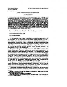
Figure 4: Last stage of a length-8 DWT based FFT. The above factorization suggests a DWT based FFT algorithm. The block diagram of the last stage of a length-8 algorithm is shown in Figure 4. Same scheme in Figure 4 are iteratively applied to shorter
length DFTs to get the full DWT based FFT algorithm. The nal system is equivalent to a full binary tree wavelet packets transform followed by classical FFT butter y operations, where the twiddle factors are the frequency response of the wavelet lters. 2
The detail of the butter y operation is shown in Figure 5, where i 2 f0; 1; : : : ; N=2 ? 1g. Now the twiddle factors are length-N DFT of h and g. For well de ned wavelet lters, they have well known properties, e.g for Daubechies' family of wavelets, their frequency responses are monotone, and nearly half of which have magnitude close to zero. This fact can be exploited to achieve speed v.s. accuracy tradeo�.
AN= (i; i)
@@ � ? CN= (i; i) @ ?? @?@? BN= (i; i) ? @ @@ ?? R 2
2
2
DN= (i; i) 2
Figure 5: Butter y operations in a radix-2 DIT FFT. The classical radix-2 DIT FFT is a special case of the above algorithm when h = [1; 0] and g = [0; 1]. Although they do not satisfy some of the conditions required for wavelets, they do constitute a legitimate (and trivial) orthogonal lter bank.
3.2 Computational Complexity For the DWT based FFT algorithm, the computational complexity is also O(N log N ), since the recursive relation in Equation 2 is again satis ed. However, the constant appears before N log N depends on the wavelet lters used. 2
2
4 Fast Approximate Fourier Transform 4.1 Basic Idea The basic idea of the fast approximate Fourier transform (FAFT) is pruning, i.e. cut o� part of the diagram. Traditionally, when only part of the inputs are non-zero, or only part of the outputs are required, the part of the FFT diagram where either the inputs are zero or the outputs are undesired is pruned, so that the computational complexity is reduced. However, the classical pruning algorithm is quite restrictive, since for majority of the applications, both the inputs and the outputs are of full length. 11
The structure of the DWT based FFT algorithm can be exploited to generalize the classical pruning idea for arbitrary signals. From the input data side, the signals are made sparse by the wavelet transform, thus approximation can be made to speed up the algorithm by dropping the insigni cant data. In other words, although the input signal are normally not sparse, DWT creates the sparse inputs for the butter y stages of the FFT. So any scheme to prune the butter y stages for the classical FFT can be used here. Of course, the price we have to pay here is the computational complexity of the DWT operations. In actual implementation, the wavelets in use have to be carefully chosen to balance the bene t of the pruning and the price of the transform. Clearly, the optimal choice depends on the class of the data we would encounter. 8,6,7,4
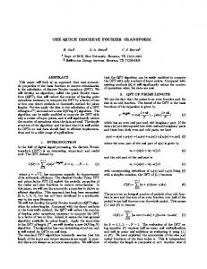
From the transform side, since the twiddle factors of the new algorithm have decreasing magnitudes, approximation can be made to speed up the algorithm by pruning the sections of the algorithm which correspond to the insigni cant twiddle factors. The frequency response of the Daubechies' wavelets are shown in Figure 6. As we can see that they are monotone decreasing. As the length increases, more and more points are close to zero. It should be noted that those lters are not designed for frequency responses. They are designed for atness at 0 and �. Various methods can be used to design wavelets or orthogonal lter banks to achieve better frequency responses. Again, there is a tradeo� between the good frequency response of the longer lters and the higher complexity required by the longer lters. 9,10,13
frequency response of Daubechies family of wavelets 1.5
length−4 length−8 length−16 length−32
magnitude
1
0.5
0 0
0.1
0.2
0.3
0.4 0.5 0.6 frequency (ω/π)
0.7
0.8
0.9
1
Figure 6: The frequency responses of Daubechies' family of wavelets.
4.2 Computational Complexity The wavelet coe�cients are mostly sparse, so the input of the shorter DFTs are sparse. If the implementation scales well with respect to the percentage of the signi cant input, e.g. it uses half of the time if only half of the inputs are signi cant, then we can further lower the complexity. Assume for
N inputs, �N of them are signi cant (� � 1), we have CFAFT (N ) = O(N ) + 2�CFAFT (N=2):
(13)
For example if � = , Equation (13) simpli es to 1
2
CFAFT (N ) = O(N ) + CFAFT (N=2);
(14)
which leads to
CFAFT (N ) = O(N ): (15) So under above conditions, we have a linear complexity approximate FFT. Of course, the complexity depends on the input data, the wavelets we use, the threshold value used to drop insigni cant data, and the threshold value used to prune the butter y operations. Good tradeo� need to be found. Also the implementation would be more complicated than the classical FFT.
5 Noise Reduction Capacity It has been shown that the thresholding of wavelet coe�cient has near optimal noise reduction property for many classes of signals. The thresholding scheme used in the approximation in the proposed FAFT algorithm is the exactly the hard thresholding scheme used to denoise the data. Soft thresholding can also be easily embedded in the FAFT. Thus the proposed algorithm also reduces the noise while doing approximation. If we need to compute the DFT of noisy signals, the proposed algorithm not only can reduce the numerical complexity, but also can produce cleaner results. 5
6 Summary In the past, FFT has been used to calculate DWT, which leads to e�cient algorithm when lters are in nite impulse response (IIR). In this paper, we did just the opposite { using DWT to calculate FFT. We have shown that when no intermediate coe�cients are dropped and no approximations are made, the proposed algorithm computes the exact result, and its computational complexity is on the same order of the FFT, i.e. O(N log N ). The advantage of our algorithm is two fold. From the input data side, the signals are made sparse by the wavelet transform, thus approximation can be made to speed up the algorithm by dropping the insigni cant data. From the transform side, since the twiddle factors of the new algorithm have decreasing magnitudes, approximation can be made to speed up the algorithm by pruning the section of the algorithm which corresponds to the insigni cant twiddle factors. 14,12,13
2
In summary, we proposed a novel fast approximate Fourier transform algorithm using the wavelet transform. Since wavelets are the conditional basis of many classes of signals the algorithm is very e�cient and has builtin denoising capacity. 12,7,4
7 REFERENCES [1] C. S. Burrus and T. W. Parks. DFT/FFT and Convolution Algorithms. John Wiley & Sons, New York, 1985. [2] R. R. Coifman and M. V. Wickerhauser. Entropy-based algorithms for best basis selection. IEEE Trans. Inform. Theory, 38(2):1713{1716, 1992. [3] I. Daubechies. Orthonormal bases of compactly supported wavelets. Comm. Pure Applied Math., XLI(41):909{996, November 1988. [4] I. Daubechies. Ten Lectures on Wavelets. SIAM, Philadelphia, PA, 1992. Notes from the 1990 CBMS-NSF Conference on Wavelets and Applications at Lowell, MA. [5] D. L. Donoho. De-noising by soft-thresholding. IEEE Trans. Inform. Theory, 41(3):613{627, May 1995. [6] Y. Meyer. L'analyses par ondelettes. Pour la Science, September 1987. [7] Y. Meyer. Ondelettes et op�erateurs. Hermann, Paris, 1990. [8] Y. Meyer. Wavelets: Algorithms and Applications. SIAM, Philadelphia, 1993. Translated by R. D. Ryan. [9] J. E. Odegard. Moments, smoothness and optimization of wavelet systems. PhD thesis, Rice University, Houston, TX 77251, USA, May 1996. [10] I. W. Selesnick. New Techniques for Digital Filter Design. PhD thesis, Rice University, 1996. [11] H. V. Sorensen and C. S. Burrus. E�cient computation of the DFT with only a subset of input or output points. IEEE Transactions on Signal Processing, 41(3):1184{1200, March 1993. [12] G. Strang and T. Nguyen. Wavelets and Filter Banks. Wellesley-Cambridge Press, Wellesley, MA, 1996. [13] P. P. Vaidyanathan. Multirate Systems and Filter Banks. Prentice Hall, Englewood Cli�s, NJ, 1992. [14] M. Vetterli and J. Kovacevic. Wavelets and Subband Coding. Prentice Hall, Englewood Cli�s, NJ, 1995.