Fast Contextual Preference Scoring of Database Tuples Kostas Stefanidis
Department of Computer Science University of Ioannina GR-45110 Ioannina, Greece
[email protected]
ABSTRACT To provide users with only relevant data from the huge amount of available information, personalization systems utilize preferences to allow users to express their interest on specific pieces of data. Most often, user preferences vary depending on the circumstances. For instance, when with friends, users may like to watch thrillers, whereas, when with their kids, they may prefer to watch cartoons. Contextual preference systems address this challenge by supporting preferences that depend on the values of contextual attributes such as the surrounding environment, time or location. In this paper, we address the problem of finding interesting data items based on contextual preferences that assign interest scores to pieces of data based on context. To this end, we propose a number of pre-processing steps. Instead of pre-computing scores for all data items under all potential context states, we exploit the hierarchical nature of context attributes to identify representative context states. Furthermore, we introduce a method for grouping preferences based on the similarity of the scores that they produce. This method uses a bitmap representation of preferences and scores with various levels of precision that lead to approximate rankings with different degrees of accuracy. We evaluate our approach using both real and synthetic data sets and present experimental results showing the quality of the scores attained using our methods.
1.
INTRODUCTION
Personalization systems aim at providing users with only the data that is of interest to them from the huge volume of available information. Preferences have been used as a means to address this challenge. To this end, a variety of preference models have been proposed most of which follow either a quantitative or a qualitative approach. With the quantitative approach (e.g., [4, 15, 17, 18]), users employ scoring functions that associate a numerical score with specific pieces of data to indicate their interest in them. With the qualitative approach (such as the work in [8, 16]), pref-
Permission to make digital or hard copies of all or part of this work for personal or classroom use is granted without fee provided that copies are not made or distributed for profit or commercial advantage and that copies bear this notice and the full citation on the first page. To copy otherwise, to republish, to post on servers or to redistribute to lists, requires prior specific permission and/or a fee. EDBT’08, March 25–30, 2008, Nantes, France. Copyright 2008 ACM 978-1-59593-926-5/08/0003 ...$5.00.
Evaggelia Pitoura
Department of Computer Science University of Ioannina GR-45110 Ioannina, Greece
[email protected]
erences between two pieces of data are specified directly, typically using binary preference relations. To enhance the expressiveness of preference models, contextual preferences have recently attracted considerable attention motivated by the fact that preferences may depend on context. Context is a general term used to express the situation of the user at the time of the submission of a query, including the surrounding environment, time or location [9]. Contextual preference models have been introduced following both the quantitative [25, 26] and the qualitative [3, 14] approach. Knowledge-based contextual preferences have also been proposed [27]. In this paper, we use context to indicate any attribute that is not part of the database schema. As our running example, we use a movie database. Users express their preferences on movie attributes. These preferences may for example depend on who is accompanying the user or the user’s age or sex. For instance cartoons may be a reasonable choice when with family, while a romantic comedy may be preferable when on a date. To allow more flexibility in describing context, we assume as in [26], that contextual attributes take values from hierarchical domains. We address the problem of scoring database tuples based on contextual quantitative preferences. In particular, given a set of contextual preferences P , a database instance r and a query q, we are interested in providing the user with the most preferable tuples in r for the current context. Assuming that the database is large and only a few tuples are of interest at any given context, sorting the whole database for each query and context will result in both wasting resources and slow query responses. Thus, we propose preprocessing steps that can be used to reduce the online time for processing each query. At one extreme, we could compute all different scores for each tuple for all potential context states. Since, only a few tuples may be of interest at each context state, we propose computing scores only for relevant tuples (i.e., tuples for which there is sufficient interest). However, the number of potential scores may be still large, since the number of context states grows rapidly with the number of context attributes. For many application, context includes a large number of attributes with domains of varying sizes. For instance, in a pervasive environment, a media player system for movies and television programs may suggest interesting programs to users according to their current context that includes their age, sex, taste as well as time, location, surrounding people, emotional state and the technical characteristics of the targeted device for playing the program. Thus, we propose computing scores only for representative
context states. Our method for identifying context representatives exploits the hierarchical nature of context attributes and can be applied to both quantitative and qualitative preferences. We also consider a complementary method for grouping preferences based on identifying those preferences that result in similar scores for all database tuples. This method takes advantages of the quantitative nature of preferences and groups together contextual preferences that have similar predicates and scores. The method is based on a novel representation of preferences through a predicate bitmap table whose size depends on the desired precision of the resulting scoring. In summary, in this paper, we make the following contributions: • We propose a suite of techniques for quickly providing users with data of interest in the case of contextual quantitative preferences. • We consider a contextual clustering method that exploits the hierarchical nature of context attributes. • We introduce a method for grouping those preferences that produce similar scores for all database tuples. The method is based on a bitmap representation with tunable accuracy. Finally, we present a number of experiments on both synthetic and real data sets. The rest of this paper is structured as follows. In Section 2, we introduce the problem of scoring database tuples based on contextual quantitative preferences. Section 3 proposes a method for finding representative context states by exploiting the hierarchical nature of context attributes, while Section 4 focuses on grouping preferences by identifying those that result in similar scores. Section 5 discusses issues of handling the produced scores. In Section 6, we present our evaluation results. Section 7 describes related work, and finally, Section 8 concludes the paper with a summary of our contributions.
2.
CONTEXTUAL PREFERENCE RANKING
In this section, we present our contextual preference model and introduce the problem of scoring database tuples using contextual preferences. As a running example, we consider a simple movie database with schema: Movie(title, year, director, genre, language, duration).
2.1
Contextual Preference Model
To model context, we use a finite set of special-purpose attributes, called context parameters. We distinguish between two types of context parameters: simple and composite ones. A simple context parameter involves a single context attribute Ci with domain dom(Ci ), while a composite context parameter Cj consists of a set of single context attributes Cj1 , Cj2 , . . . , Cjl with domains dom(Cj1 ), dom(Cj2 ), . . . , dom(Cjl ), respectively and its domain, dom(Cj ) is equal to dom(Cj1 ) × dom(Cj2 ) . . . × dom(Cjl ). For a given application X, we define its context environment CEX as a set of n context parameters {C1 , C2 , . . . , Cn }. In our running movie example, we consider the simple context parameters accompanying_people, time_period and mood. We also
consider users to be part of context, so that the result of each query depends on the user submitting it. Each user is modeled by the composite context parameter user consisting of attributes id, age and sex. Thus, our context environment is the quadruple (user, accompanying_people, time_period, mood). Similar to [26], context attributes take values for multidimensional domains. In particular, we assume that each context attribute participates in an associated hierarchy of levels of aggregated data, i.e., it can be viewed using different levels of abstraction. Formally, an attribute hierarchy is a lattice (L, ≺): L = (L1 , . . . , Lm−1 , ALL) of m levels and ≺ is a partial order among the levels of L such that L1 ≺ Li ≺ ALL, for every 1 < i < m. We require that the upper bound of the lattice is always the level ALL, so that we can group all values into the single value ‘all’. We use the notation domLj (Ci ) for the domain of level Lj of attribute Ci . Figure 1 depicts the hierarchies of the context attributes for our example. Such hierarchies may be constructed using for example the WordNet [20] or related ontologies. A function L ancLkj assigns a value of the domain of Lj to a value of the
2 domain of Lk . For instance, ancL L1 (Christmas) = holidays. Hierarchies support the specification of context values with various levels of detail. For a context environment with n context attributes, a context state cs is a n–tuple of the form (c1 , c2 , . . . , cn ), where ci ∈ dom(Ci ). For example, a context state in our example may be ((all, youth, male), f riends, T h, good) or ((id1, middle_age, f emale), f amily, holidays, good). To specify preferences, we use a simple quantitative preference model similar to the ones in [4, 26]. In particular, users express their preference for sets of tuples specified using selection conditions on some of the attributes of the tuples by rating them using a numerical score. The score is a real number between 0 and 1 which expresses their degree of interest for the specified tuples. Value 1 indicates extreme interest, while value 0 indicates no interest. Preferences are annotated with context information to denote the context state in which the preference holds.
Definition 1 (Contextual Preference). Given a database schema R(A1 , A2 , . . . , Ad ), a contextual preference p on R is a triple (cs, P red, score), where cs is a context state, P red is a predicate of the form Ai1 θ1 ai1 ∧ Ai2 θ2 ai2 . . . ∧ Aik θk aik that specifies conditions θi on the values aij ∈ dom(Aij ) of attributes Aij , 1 ≤ ij ≤ d, of R, and score is a real number between 0 and 1. The meaning of such a contextual preference is that in context state cs, all database tuples t for which P red holds are assigned the indicated score. In our running example, we assume θ ∈ {=, , ≤, ≥, 6=} for the attributes year and duration and θ ∈ {=} for the remaining attributes. For instance, a preference (((id1, youth, male), f riends, holidays, good), (genre = comedy), 0.9) denotes that user with id id1 who is a young male, when accompanied with f riends during holidays and in good mood enjoys seeing movies of genre comedy. Note that it is not necessary for a preference to depend on all context attributes. This can be expressed by assigning the value all to the corresponding context attribute. For instance the preference (((all, youth, all)), all, holidays, all), (genre = comedy), 0.9) means that all young people
Accompanying_people All (L2)
friends, family, alone, date (L1) Mood All (L2)
Time_of_life All (L2)
Time_period All (L3)
Working_days, Weekend,
Holidays (L2)
youth, middle_age, old_age (L1) Sex All (L2)
M, Tu, W, Th, F Sa, Su
Summer, Christmas, Easter (L1) male, female (L1)
good, bad, indiferrent (L1)
Figure 1: Context Hierarchies. like to see comedies during holidays independently of the values of the other context parameters. For simplicity, in the following, we shall skip all values in the context part of the preference and for example, simply use ((youth, holidays), (genre = comedy), 0.9) to express the preference above. We call the set of contextual preferences that hold for an application, profile P . By CS(P ), we denote the set of context states cs that appear in at least one preference in P . We assume that such profiles are available. In practice, preferences may be, for example, given by the users explicitly or may be deduced by say the previous behavior of the same or similar users. A practical way to create P , considered in [26], is by assembling a number of default profiles and allowing users to update them appropriately.
2.2
Computing Interest Scores
Given a set of preferences specified in a profile P , we associate an interest score for each tuple t of any instance r of R, for each context state cs ∈ CS(P ). In this section, we specify how. If none of the preferences specified for context state cs are applicable to a tuple t, that is, the corresponding predicates in the preferences defined for cs do not hold for t, then t is assigned a default score of 0. This is because, we consider preferences expressed by users to be indicators of positive interest. Consequently, we assume that an unrated tuple is less important than any other tuple for which the user has expressed some interest. There may be more than one preference applicable to a specific database tuple t. In other words, a tuple t may satisfy the predicate part P red of more than one of the preferences specified for context state cs. In general, if more than one preference is applicable to a tuple, we choose the one with the highest score, except when the predicates of the preferences are related in the following sense. We use the notation P red[t] to denote that predicate P red holds for tuple t. Assuming two predicates P red1 and P red2 , we say that P red1 subsumes P red2 , iff ∀ t ∈ r, P red1 [t] ⇒ P red2 [t], which means that P red1 is more specific than P red2 . When a tuple satisfies predicates that one subsumes the other, to compute its score, we consider only the preferences with the most specific predicates, because these are considered as used by the users to specialize or refine the general ones. Definition 2 (Tuple Score). Let P be a profile, cs a context state and t ∈ r a tuple. Let P 0 ⊆ P be the set of preferences pi = (cs, P redi , scorei ), such that, P redi [t] holds and ¬ ∃ pj = (cs, P redj , scorej ) ∈ P 0 , such that,
P redj subsumes any P redi . The score of t in cs, score(t, cs), is defined as follows: P 0 6= ∅ maxpi ∈P 0 scorei , score(t, cs) = 0, otherwise For example, assume the movie relation of Table 1 and a profile with the following simple preferences: p1 = ((f riends), genre = horror, 0.8), p2 = ((f riends), director = Hitscock, 0.7), p3 = ((alone), genre = drama, 0.9), p4 = ((alone), (genre = drama ∧ director = Spielberg), 0.5). In context f riends, both preferences p1 and p2 are applicable to t2 . Similarly, both preferences p3 , p4 are applicable to tuple t3 in context alone. In the first case, none of the two predicates subsumes the other and the score for t2 is the maximum of the two scores, namely 0.8. Under context alone, the predicate of p4 subsumes the predicate of p3 , and so, t3 has score 0.5. The reason is that the user has assigned score 0.9 to drama movies in general and score 0.5 to drama movies directed by Spielberg. Tuple t3 belongs to the second category and thus it is assigned the corresponding most specific score. As another example of more than one preference applicable to a database tuple consider the following. Assume that a user defines that she prefers to watch horror movies at the weekend and rates such movies with a high score of 0.9. If later on, she adds a second preference, assigning to Hitchcock movies under context weekend an interest score of 0.3, this will cause some kind of conflict, since two different scores are assigned to the movie P sycho (Table 1) in the same context. However, from the way the score of a tuple is computed (Def. 2), such conflicts are resolved implicitly by taking the maximum score among all relative scores (score 0.9 in this example), considering contextual preferences as indicators of positive interest. Note that, as in the previous Spielberg example, if the user wanted to “exclude” horror movies by Hitchcock, she could use in her second preference the most specific predicate genre = horror ∧ director = Hitchcock instead of just director = Hitchcock. Clearly, one could argue for other types of combining preferences, besides “max”, for instance, using “min” or a weighed sum. Our main motivation is that we treat preferences as indicators of positive interest. By using “max”, we may overrate a database tuple, resulting in some form of a false positive, but we never miss interesting data items.
2.3
Problem Formulation
Each query submitted by a user is associated with one or more context states. Typically, the context implicitly asso-
t1 t2 t3
T itle Casablanca Psycho Schindler’s List
Table 1: Database Instance Y ear Director Genre Language 1942 Curtiz Drama English 1960 Hitchcock Horror English 1993 Spielberg Drama English
ciated with a query corresponds to the current context, that is, the context surrounding the user at query submission time. To capture the current context, many context-aware applications use various devices for determining the values of the relevant context parameters such as temperature sensors or GPS-enabled devices for location-related attributes. Besides such implicit context augmentation, queries may be explicitly enhanced with context states for example for posing exploratory queries such as what is a good movie to watch with my family this coming weekend. Now given the query context states CSq of a query q, we would like (1) to identify the set Pq ⊆ P of preferences (cs, P red, score) for which cs = csq , for some csq ∈ CSq , and then, (2) use them to compute a score for each tuple t in the result of q. The first problem is complicated by the fact that for some csq in CSq , there may be no preference (cs, P red, score) in the profile P , with cs = csq , that is csq ∈ / CS(P ). Note, that the set of all possible context states for a context environment with n parameters is equal to |dom(C1 )| × |dom(C2 )| × . . . |dom(Cn )|. In practice, the profile contains preferences only for a small number of such states. To address this, we use those preferences in P that have the most similar context states. That is, for each query context state csq , we use the preferences (cs, P red, score) in P with mincs ∈ CS(P ) distS (cs, csq ). We defer the definition of distance distS between context states to Section 3.1. Next, we define the score of a tuple with regards to a set of context states:
database and that only a few tuples are of interest at any given context, computing a score for all database tuples for each context state will result in both wasting resources and slow query responses. Since, the number of possible context states grows rapidly with the number of context attributes, we could instead compute the scores for all states that appear in the profile and then combine the scores of the most similar ones online. Since the number of context states that appear in a profile can still be large, we propose two approaches for finding representative scores to precompute. The first approach constructs clusters of preferences, considering as similar those preferences that have either the same or similar context states. The second one clusters preferences that lead to similar scores for database tuples. After constructing the clusters of preferences, we compute for each cluster, an interest score for each database tuple using the preferences of this cluster. Furthermore, instead of storing scores for all database tuples for each cluster, we just store the nonzero ones. Then, for each query, we can search for the most similar to the query cluster and quickly provide the best results, that is, the results with the largest scores. In a nutshell, our solution framework for addressing the above problem consists of the following components: 1. Having defined preferences that hold under different circumstances, we cluster them according either to (a) their context part, thus creating clusters of preferences applicable to similar context states, or (b) their non-context part (i.e., the predicate and score part), thus creating clusters of preferences that produce similar scores.
Definition 3 (Aggregate Tuple Score). Let P be a profile, CS ⊆ CS(P ) be a set of context states and t ∈ r a tuple. The aggregate score of t in CS is: score(t, CS) = maxcs∈CS score(t, cs).
2. Using the preferences of each cluster, we compute an interest score for each tuple for the given cluster. 3. For a submitted query, we search for the most similar to the context of the query clusters. Using the scores of tuples of the returned clusters, we quickly rank the results based on the computed scores.
Now, the second problem can be expressed as follows: Problem Definition. Assume a database instance r, a profile P and a query q with a set of context states CSq . Let CS ⊆ CS(P ) be the set of context states cs with the minimum distS (cs, csq ), csq ∈ CSq , that is, the context states that are the most similar to the context states of the query. The contextual scoring problem is to rank all tuples t in the result of q based on the aggregate score score(t, CS). For computing the scores of all tuples in the result set, a solution that involves no pre-computation is to first find the set of context states CSq , compute the scores of all tuples t in the result and then rank them based on these scores. Performance can be improved by performing preprocessing steps offline. One approach would be to compute the scores of each tuple for each potential context state. Assuming a large
Duration 102 109 195
In the following two sections, we describe how we cluster preferences for the case of context state similarity and the case of predicate similarity.
3.
FINDING REPRESENTATIVE CONTEXT STATES
Instead of computing aggregate scores for all tuples for all potential context states, we identify representative context states and pre-compute scores according to them. Computing interest scores using only representative context states is based on the assumption that preferences defined for similar context states would result in producing similar scores for most tuples.
In the following, we first define the notion of similarity or, equivalently, distance between context states. Then, we use a simple clustering algorithm that groups similar context states and selects one context state per cluster as a representative state.
3.1
Similarity between Context States
Defining similarity between context states is a difficult problem, since context similarity is in general application dependent. Here, we take a rather generic, syntactic approach that exploits the hierarchical domains of each context parameter. First, we define similarity for each of the context parameters. A direct method to compute the distance between two values of a context parameter is by relating their distance with the length of the minimum path that connects them in their associated hierarchy. However, this method may not be accurate, when applied to attributes with large domains and many hierarchy levels. This is because values in upper levels of the hierarchy are intuitively less similar than values in lower levels connected with paths of the same length. For instance, in our simple example of the T ime_period hierarchy, when considering only the path length, values T u and W have the same distance with each other as value W orking_days has with W eekend. Moreover, the distance between T u and W is the same as T u and all, whereas, T u is intuitively more similar to W than to all. Following related research on defining semantic similarity between terms (e.g., [19]), in defining the distance between two values of a context parameter, we take into account both their path distance and the depth of the hierarchy levels that the two values belong to. Let lca(c1 , c2 ) be the lowest common ancestor of context values c1 and c2 . The path and depth distance between two values are defined as follows. Definition 4 (Path distance). The path distance distP (c1 , c2 ) between two context values c1 ∈ domLj (Ci ) and c2 ∈ domLk (Ci ): • is equal to 0, if c1 = c2 , • is equal to 1, if c1 , c2 are values of the lowest hierarchy level and lca(c1 , c2 ) is the root value of their corresponding hierarchy, • or is computed through the fp function (1 − e−α×ρ ), where α > 0 is a constant and ρ is the minimum path length connecting them in the associated hierarchy. The fp function is a monotonically increasing function that increases as the path length becomes larger. The above definition of path distance ensures also that the distance is normalized in [0, 1]. Definition 5 (Depth distance). The depth distance distD (c1 , c2 ) between two context values c1 ∈ domLj (Ci ) and c2 ∈ domLk (Ci ): • is equal to 0, if c1 = c2 , • is equal to 1, if lca(c1 , c2 ) is the root value of their corresponding hierarchy, • or is computed through the fd function (1 − e−β/γ ), where β > 0 is a constant and γ is the minimum path length between the lca(c1 , c2 ) value and the root value of the corresponding hierarchy.
The fd function is a monotonically increasing function of the depth of the lowest common ancestor. Again, the definition of depth distance ensures distances within the range [0, 1]. Having defined the path and the depth distances between two context values, we define next their overall distance. Definition 6 (Value distance). The value distance between two context values c1 and c2 is computed as: distV (c1 , c2 ) = distP (c1 , c2 ) × distD (c1 , c2 ). For example, the path distance between values summer and working_days is 1 − e−3 ' 0.95, their depth distance is 1, and so, their value distance is 1 × 0.95 = 0.95. Whereas values holidays and summer have value distance equal to (1 − e−1×1 ) × (1 − e−1/1 ) ' 0.39. This means that the value summer is more closely related to holidays than to working_days as expected. In both examples, we assume that α = β = 1. Note that to compute the value distance distV , we use the independent distP and distD distances. This independence enables us to combine them in different ways by giving different weights of interest. To do this, we may assign different values to the constants α, β. In particular, for constant values greater than 1, the corresponding distance increases, while values within the range (0, 1) result in smaller distances. Having defined the distance between two context values, we can now define the distance between two context states. To achieve this, we use a simple weighted sum, but other methods of aggregation are also possible. Definition 7 (State distance). Given two context states cs1 = (c11 , c12 , . . . , c1n ) and cs2 = (c21 , c22 , . . . , c2n ), the state distance is defined as:P 1 2 distS (cs1 , cs2 ) = n i=1 wi × distV (ci , ci ), where each wi is a context parameter specific weight. P The above weights are normalized, such that, n i=1 wi = 1. The weight assigned to each context parameter is application dependent, since for some applications, some context parameters may be more influential than others. Again, in this paper, we take a generic approach and assign weights to each context parameter according to the cardinality of its domain. In particular, we assign larger weights to parameters with smaller domains, considering a higher degree of similarity among values that belong to a large domain. It is easy to show that the distance relationship between context states is reflexive (distS (cs1 , cs1 ) = 0), and symmetric (distS (cs1 , cs2 ) = distS (cs2 , cs1 )). However, it does not satisfy the triangle inequality (distS (cs1 , cs2 ) ≤ distS (cs1 , cs3 ) + distS (cs3 , cs2 )), because of the semantic way of defining distances among context values, as the following example shows. Assume 3 context states cs1 , cs2 , cs3 with a single context parameter, say T ime_period, and in particular, cs1 = (Sunday), cs2 = (Summer), cs3 = (All). Assuming further that α, β are equal to 1, distS (cs1 , cs2 ) ≤ distS (cs1 , cs3 ) + distS (cs3 , cs2 ) does not hold, because 1 ≤ (1 − e−2 ) + (1 − e−2 ) does not hold.
3.2
Contextual Clustering
To group preferences with similar context states, we use a typical hierarchical agglomerative clustering method that follows a bottom-up strategy. Initially, the d-max algorithm
(Algorithm 1) places each context state in a cluster of its own. Then, at each step, it merges the two clusters with the smallest distance. The distance between two clusters is defined as the maximum distance between any two context states that belong to these clusters. The algorithm terminates when the closest two clusters, i.e., the clusters with the minimum distance, have distance greater than dcl , where dcl is an input parameter. Finally, for each produced cluster, we select as representative context state, the state in the cluster that has the smallest total distance from all the states in its cluster. Formally: Definition 8 (Representative context state). Let cli be a cluster produced by the d-max algorithm that consists of a set CScli of m context states, csij . The representative of Pmcli is the context state cs ∈ CScli , with the minimum j=1 distS (cs, csij ) value.
Algorithm 1 d-max Algorithm Input: A set of preferences with context states csi , a distance value dcl . Output: A set of clusters. Begin 1. Create a cluster for each context state csi . 2. Repeat. 2.1 If the minimum distance among any pair of clusters is smaller than dcl . 2.1.1 Merge these two clusters. 2.2 Else, end loop. 3. Compute the representative context state of each produced cluster. End Using the d-max algorithm, any two context states cs1 , cs2 that belong to the same cluster have distance distS (cs1 , cs2 ) ≤ dcl . Therefore, the following property holds. Property 1. Given a cluster distance dcl , each cluster cl produced by the d-max algorithm has context states, such that, any pair of context states cs1 , cs2 ∈ cl have distance distS (cs1 , cs2 ) ≤ dcl . Proof: From step 2, of the d-max algorithm, we merge the closest two clusters, if their distance is less or equal to dcl . This distance represents the maximum distance between a context state cs1 of the first cluster and a context state cs2 of the second one. Therefore, any two context states cs1 , cs2 that belong to the same cluster, have distance distS (cs1 , cs2 ) ≤ dcl . 2 After generating the clusters of preferences, we compute for each of them an aggregate score for each tuple specified in any of its preferences (using the definition of the aggregate tuple score). For each produced cluster cli , we maintain a table, called scoring table, cli Scores(tuple_id, score), in which we store in decreasing order only the scores of tuples that satisfy at least one of the predicates in the preferences of the cluster. That is, we do not maintain scores for all tuples, but only for those having nonzero scores. Each time a query is submitted, we search for the most similar cluster or clusters, that means, for the clusters whose representative context state is the most similar to the query context. Then,
using the scoring table of the corresponding clusters, we can quickly retrieve the tuples with the highest scores. It is straightforward (by Definition 3) that: Property 2. Let cs be a context state and CS a set of context states. If cs ∈ CS, then for any t ∈ r, score(t, CS) ≥ score(t, cs). This means that the score of a tuple computed using the representative context state is no less than the score of the tuple computed using any of the context states belonging to the cluster. In other words, if the context state that is the most similar to the query context belongs to the cluster whose representative context state is the most similar to the query, then the score that our approximation approach computes for a tuple cannot be lower than the exact one. That is, we may overrate a tuple, but we never underrate it.
4. PREDICATE CLUSTERING Context-based clustering groups together similar context states. In this section, we consider an alternative approach for clustering context states that aims at grouping together context states that produce similar scores for most database tuples. To this end, we introduce a bitmap representation for the preferences applicable to a context state cs. Let P be the set of all predicates that appear in P and l be the number of all distinct scores. We define the preference matrix B(cs) for a context state cs as an l × |P| two-dimensional array, where B(cs)[i, j] = 1, if and only if, there is a preference that holds under context cs and gives to tuples for which predicate j holds an interest score equal to i. In particular: Definition 9 (Preference matrix). A preference matrix B(cs) for a context state cs is a bitmap l × |P| array, where |P| is the number of all distinct predicates and l the number of all distinct scores in P , such that, B(cs)[i, j] = 1, if and only if, there is a preference (cs, j, i) ∈ P . Clearly, if the matrices B(cs1 ) and B(cs2 ) of two context states cs1 and cs2 are the same, then all database tuples have the same scores for context states cs1 and cs2 . Since these preference matrices can be very large, we define approximations of them as follows. Definition 10 (Predicate representation). A predicate representation of a context state cs and score s, BV (cs, s), 0 ≤ s ≤ 1, is a binary vector of size |P|, such that, BV (cs, s)[j] = BORi≥s B(cs)[i, j], where BOR is the binary OR operation. This means that if B(cs, s)[j] = 1, then the score of every tuple t for which predicate j is true has score in context state cs at least equal to s, that is, Property 3. Let BV (cs, s) be the predicate representation for context state cs and score s. If BV (cs, s)[j] = 1 ⇒ ∀ t ∈ r, for which predicate j holds, score(t, cs) ≥ s. Proof: Assume that BV (cs, s)[j] = 1. From Definition 10, this means that, for some i, i ≥ s, B(cs)[i, j] = 1. Thus, from Definition 9, a preference (cs, j, i) belongs to P , thus from the definition of contextual preferences, for each tuple
t for which preference j holds, score(t, cs) ≥ i, which proves the property. 2 Based on this property, the following properties relate the predicate representations for two context states cs1 and cs2 with the interest scores they assign to tuples.
Table 2: BM for f riends horror Hitscock Spielberg 0.8 1 0 0 0.7 1 1 0 0.6 1 1 0
Property 4. Let BV (cs1 , s) and BV (cs2 , s) be the predicate representations of two context states cs1 and cs2 for score s. (a) If ∀ j, BV (cs1 , s)[j] = 1 ⇒ BV (cs2 , s)[j] = 1, then the set of tuples that have score larger than s in cs2 is a superset of the set of tuples that have score larger than s in cs1 . (b) If ∀ j, BV (cs1 , s)[j] = 1 ⇔ BV (cs2 , s)[j] = 1, then the set of tuples with scores larger or equal to s are the same in both context states. Proof: Proof of (a): Let t be a tuple that has score larger than s in cs1 , score(t, cs1 ) ≥ s. This means that there is at least one preference (cs1 , j, s0 ) with s0 ≥ s that belongs to profile P , for which predicate j holds in t. From Definition 10, this means that for this j, BV (cs1 , s)[j] = 1. Thus, BV (cs2 , s)[j] = 1, and from Property 3, it holds score(t, cs2 ) ≥ s. Proof of (b): This holds trivially from (a). 2 The distance between two binary vectors depends on the number of bits they differ at. In particular, letPV1 and V2 be two binary vectors of size m, then dif f = m i=1 |V1 (i) - V2 (i)|. For computing the distance between two binary vectors, we shall use the well known Jaccard coefficient that ignores the negative matches, that is, the bits for which both vectors have values equal to 0. Let pos be the number of bits that are equal to 1 for both V1 and V2 . Definition 11 (Vector distance). The distance of two vectors V1 and V2 of size m is equal to: f distV (V1 , V2 ) = difdif , if dif f +pos 6= 0 and 1 otherwise. f +pos It is clear that given two context states, the number of bits that their predicate representations differ at is an indication of the number of tuples that they rank differently. Specifically, from Property 4(b), if for two context states cs1 and cs2 , distV (BV (cs1 , s), BV (cs2 , s)) = 0, then the set of tuples with score greater or equal to s associated with each BV is the same. Note that some predicates may hold for more tuples than others. If such information regarding the selectivity of the predicates is available or can be estimated, then it P is possible m to consider a weighted version of dif f as follows: i=1 w(i) |V1 (i) - V2 (i)|, where each w(i) is set to be proportional to the selectivity of the predicate i. Now, instead of storing bitmap representation vectors BV for all distinct interest scores si , we create an overall bitmap representation matrix BM with only b rows, one for each score s1 , s2 , . . . , sb , with 0 ≤ s1 < s2 < . . . < sb ≤ 1. In particular: Definition 12 (Overall predicate representation). An overall predicate representation matrix BM for a context state cs and b scores s1 , s2 , . . . , sb , with 0 ≤ s1 < s2 < . . . < sb ≤ 1 is a bitmap b × |P| array, where |P| is the number of predicates in P , such that, BM (cs)[i, j] = BV (cs, si )[j], 1 ≤ i ≤ b, 1 ≤ j ≤ |P|.
0.8 0.7 0.6
Table 3: BM for alone horror Hitscock Spielberg 0 0 0 1 0 0 1 0 1
Simple overall predicate representation matrices with b = 3 for the preferences: p1 = (friends, genre = horror, 0.8), p2 = (friends, director = Hitscock, 0.7), p3 = (alone, genre = horror, 0.7) and p4 = (alone, director = Spielberg, 0.6), are depicted in Tables 2 and 3. Next, we define the distance between two such predicate representation matrices: Definition 13 (Overall representation distance). The distance between two overall predicate representation b × |P| matrices BM (cs1 ) and BM (cs2 ) of two context states cs1 and cs2 , is defined as: distBM (BM (cs1 ), BM (cs2 )) = Pb
i=1
distV (BV (cs1 ,si ),BV (cs2 ,si )) . b
For instance, the distance between the matrices that are shown in Tables 2 and 3 is equal to: 1+1/2+2/3 = 13 . Note 3 18 that the distance between overall representation matrices takes values within the range [0, 1]. For the distance among any predicate representation matrices BM1 , BM2 and BM3 , the following properties hold: 1. distBM (BM1 , BM1 ) = 0 (reflexivity); 2. distBM (BM1 , BM2 ) = distBM (BM2 , BM1 ) (symmetry); 3. distBM (BM1 , BM2 ) ≤ distBM (BM1 , BM3 ) + distBM (BM3 , BM1 ) triangle inequality). Proof is omitted due to space limitations. Thus, the overall representation distance is a metric. We could also consider weighted versions where rows that correspond to higher scores influence the overall distance more than rows that correspond to smaller scores. Also, note that these matrices can still be very large, when the number of predicates is large. One can consider reducing the number of columns by grouping together similar predicates or by ignoring predicates with small selectivity. We leave this issue as future work. Using distances among overall predicate matrices, we create clusters of preferences that result in similar scorings of database tuples. To do this, we use the d-max algorithm. Again, initially, each preference with a specific context state is placed in its own cluster. At each step, we merge the two clusters with the smallest distance, computing the distance as in Definition 13. The distance between two clusters is defined as the maximum distance between any two overall predicate representation matrices of context states that belong to these clusters. The algorithm terminates when the
closest two clusters have distance greater or equal to scl , where scl is an input parameter. Observe that we use the predicate matrices only to group similar preferences and not for computing scores. After the clusters have been created, we compute for each cluster an aggregate score for the tuples. As in our contextual clustering method, for each cluster cli , we maintain a scoring table cli Scores(tuple_id, score), where we store in decreasing order only the scores of tuples that satisfy at least one of the predicates in the preferences of the cluster (and not the scores equal to 0). When a query is submitted, we search for the most relevant cluster or clusters, that means, for the clusters that contain the preference(s) with the same or the most similar context state (or states in the case of ties) to the query context state. From the way an aggregate tuple score is computed within a cluster, Property 2 holds. This means that, when using the predicate clustering approach, the score of a tuple is no less than the score computed using any preference of the cluster. Therefore, as with contextual clustering, we may overrate a tuple, but we never underrate it.
5.
DISCUSSION
Since there is potentially one different score for each database tuple per context state, the number of these scores and thus database rankings can be very large. So far, we have addressed the problem of reducing the number of precomputed database scores through clustering. Next, we discuss further the issue of handling the interesting rankings after they have been identified through our clustering algorithms. We also consider how to maintain the rankings in the presence of profile and database updates.
5.1
Online Phase
Once the interesting clusters and thus rankings are identified, there are many alternative ways to materialize them. Since, our focus is on determining the interesting rankings, rather than on their efficient realization, we have adopted the following simple approach. We assume that the produced scores for each interesting cluster are stored in special tables, called scoring tables, with two attributes the tuple_id and the associated score. There is one scoring table per interesting ranking, that is, per cluster. The scoring tables are sorted by score. When a contextual query q is submitted, the scoring table that is associated with its context csq is used. In the case of contextual clustering, this is the table that corresponds to the cluster whose representative context state cs is the most similar to csq . In the case of predicate clustering, we use the table corresponding to the cluster that contains either csq or if csq does not appear in the profile, the context state that is the most similar to csq . Locating the appropriate scoring table can be achieved by maintaining an additional directory table (C1 , C2 , . . . , Cn , table_id), where Ci , 1 ≤ i ≤ n, is a context attribute and table_id is the scoring table associated with the respective context state. The selection of the appropriate table can be made more efficient by deploying indexes on the context attributes that appear in the profile P . Such a prefix-based data structure, termed profile tree, was introduced in [26]. Moreover, the physical storage of the precomputed results can be improved. For instance, we can avoid computing the scores for each tuple and storing them in the scoring table.
Instead, we could simply cluster preferences in the profile P and build appropriate indexes on the database tuples based on the predicates that appear in the preferences of each cluster. For example, for each cluster, we can just index the tuples that satisfy predicates associated with high scores. In this case, again we first locate the appropriate cluster based on the context query csq . Then, we use the associated predicate indexes to find the tuples with the highest scores. When more than one cluster are used to compute the results of a query, we can use a top − k algorithm (such as, FA, TA or their variations [11, 12, 13, 21]) to combine the ordered lists maintained in the scoring tables cli Scores of the related clusters. Furthermore, we point out that in this paper, as in many search engines and similar to [3], we rank tuples independently of the specific query. Ranking the results of ad-hoc SQL queries in a context state csq can be achieved by joining their results with the scoring table applicable to the specific context state. As a final note, consider that the two clustering approaches can be applied together. For example, we can apply predicate clustering first. Then, we can apply contextual clustering to group the clusters produced based on the similarity of their context states.
5.2
Handling Updates
Precomputing results increases the efficiency of queries but introduces the overhead of maintaining the results in the presence of updates. In this section, we discuss handling insertions and deletions of contextual preferences and database tuples. An update is considered as a delete followed by an insert. When a database tuple is added (deleted), we just need to add (delete) its entries in all scoring functions. Clustering is not affected. In the case of profile updates, let us, first, consider the case of adding or deleting a preference for a context state cs that already exists, that is, for a context state for which other preferences are already in the profile. In the case of contextual clustering, the clustering itself is not affected, since it is solely based on the context states. We just need to update the scores in the scoring table of the cs cluster of all tuples affected. This may be expensive, since in the absence of indexes, this may require scanning the whole database. On the other hand, in the case of predicate clustering, adding a preference for an existing context state cs may affect clustering. This happens when the addition of the preference causes the distance of the predicate table for cs to exceed the threshold distance scl from the other tables in its cluster. This means that cs must be moved to another cluster. Again, we need to update the scores in the associated scoring table of the previous and the new cluster of cs. The same holds for the deletion of a preference. Let us now consider the addition of preferences for a new context state, ncs. In the case of contextual clustering, this requires finding an appropriate cluster for ncs and updating the associated scoring table. Analogously, in the case of predicate clustering, the predicate table for ncs is computed and ncs enters the appropriate cluster based on its predicate table. The scoring table of the cluster that received ncs must be updated in both cases. The above operations may be expensive. However, typically, updates, and especially profile updates, are not as
Table 4: Input Parameters Parameters Synthetic Data Sets Database Number of database tuples 100000 Number of relation attributes 5 Preferences Number of contextual preferences 10000 Number of context attributes 3, 4 Number of non context attributes 2 Data distribution zipf - a = 1.5 Cardinality of context domains 100 Hierarchy levels 4 Cardinality of non-context domains 50
6.
EVALUATION
Contextual clustering is based on the premise that preferences for similar context states produce similar scores. We first run a related experiment to explore this. Then, we evaluate both contextual and predicate clustering regarding the number of representative rankings and the associated accuracy using both real and synthetic datasets.
6.1
Context and Preference Similarity
The goal of this experiment is to show that often preferences for similar context states are also similar. Since there are no real large profile data sets defined using our contextual preferences, we used a real dataset of movie ratings that includes 1000 users, 4000 movies and 150000 ratings [2]. Ratings are of the form (user_id, movie_id, rating_value), with rating_value in the range [1, 5]. For users, there is information available of the form (user_id, sex, age, occupation) that we use as our context environment. We constructed simple predicates that involve the genre of the movies by averaging the rates assigned by each user to movies of each genre. We consider five values for the genre attribute namely, comedy, action, thriller, horror and drama. Using the profile such constructed, we show how preferences vary with context (i.e, user attributes). We compute the distance between two context states (users) using the distance between two context states (Def. 7) with equal weights assigned to each of the four parameters user_id, sex, age, and occupation. We compute the distance between two ratings using the overall representation distance (Def. 13). The ratings of each user are represented with an overall predicate representation 5 × 5 matrix, where there is one row for each rating (1 to 5) and one column for each movie genre. As shown in Fig. 2, the distance between ratings increases as the distance between users increases.
6.2
Contextual and Predicate Clustering
We run a set of experiments using both synthetic and real data sets to evaluate both the contextual and the predicate
40000 6 1000 3 1 3 - 15 2, 3
1 Distance between ratings
frequent as queries. Furthermore, one can consider batch variations, where updates are not applied immediately but say periodically or when their number exceeds some threshold. In between, the users get results that may be less accurate. In such cases, various optimizations are possible by aggregating the effects of a number of updates and applying them collectively.
Real Data Sets
0.8 0.6 0.4 0.2 0 0
0.2
0.4 0.6 Distance between users
0.8
1
Figure 2: Distance of rankings as a function of distance between users.
clustering approaches. In both cases, we use a variation of the d-max clustering algorithm, that uses as input the number of clusters instead of the distance. This allows us to directly relate the number of clusters with the quality of the rankings. Concerning the synthetic data sets, we use a database with 100000 tuples. The database schema consists of a single relation with 5 attributes. A synthetic profile consists of 10000 contextual preferences, each involving 3 context attributes and 2 database attributes. Context and non-context (attribute) values are selected using a zipf data distribution with a = 1.5 from context domains with 100 values and 4 hierarchy levels, and respectively, from domains with 50 values. We consider two cases for producing synthetic profiles. In the first case, there is no correlation between the context values and the other part of the preferences. In the second case, we construct correlated profiles, that is, we produce preferences for which similar context states have similar predicates and scores. Regarding the real data sets, we use a real database with information about movies from the Internet Movies Database (IMDB) [1]. In particular, we extract from IMDB movies with language English, French, Greek, German, Spanish or Japanese. Our subset consists of nearly 40000 movies. The database schema consists of a single relation: Movie(title, year, director, genre, language, duration). We run our prototype implementation for 10 users. Each user was asked to express contextual preferences for movies. To express such contextual preferences, users used the context parameters that are depicted in Fig. 1 (namely, Accompanying_people, Mood and Time_period) and 1 attribute of the movie relation. Each user provided about 100 preferences. We use
1
1 With correlation Without correlation
0.8
Distance within clusters
Distance within clusters
Contextual clustering
0.6 0.4 0.2 0
0.8 0.6 0.4 0.2 0
2
4
6
8
10 12 Num of clusters
14
16
18
20
0
100
200
300
400 500 600 Num of clusters
700
800
900
1000
Figure 3: Distance between context states within the produced clusters for the contextual clustering approach, for real (left) and synthetic data sets (right). 1 Predicate clustering (4 rows) Predicate clustering (5 rows) Predicate clustering (5 rows with weights)
0.8
Distance within clusters
Distance within clusters
1
0.6 0.4 0.2 0
With correlation (4 rows) With correlation (5 rows) With correlation (5 rows with weights) Without correlation (4 rows) Without correlation (5 rows) Without correlation (5 rows with weights)
0.8 0.6 0.4 0.2 0
2
4
6
8
10 12 Num of clusters
14
16
18
20
0
100
200
300
400 500 600 Num of clusters
700
800
900
1000
Figure 4: Distance between context states within the produced clusters for the predicate clustering approach, for real (left) and synthetic data sets (right). these preferences to construct a real profile having nearly 1000 preferences. Our input parameters are summarized in Table 4. We count the average distance within the produced clusters using the d-max clustering algorithm for different number of produced clusters (Experiment I ). This is an indication of the similarity of the preferences that belong to the same cluster. Then, we evaluate the quality of the returned results for a query (Experiment II ).
Experiment I. In this set of experiments, we vary the maximum number of clusters (i.e., rankings) and report the average distance between context states within each cluster for the contextual clustering approach and the average overall representation distance within each cluster for the predicate clustering approach. Figure 3 reports the average distance among context states within the produced clusters for the contextual clustering approach for the real preferences (Fig. 3 (left)) and for the synthetic ones (correlated and non-correlated case) (Fig. 3 (right)). As expected, the correlation between the contextual and the non contextual part of a preference does not affect the distance between the context states, since contextual clustering just uses the context part. For both the synthetic and the real data sets, the distance decreases with the number of clusters. Note that when using real preferences, the number of rankings (resp., clusters) is small because of the small cardinalities of context domains and the high degree of similarity among user preferences. Figure 4 depicts results for the predicate clustering approach for different values of b, where b is the number of rows (scores) of the predicate matrix for the same real (Fig. 4 (left)) and synthetic (Fig. 4 (right)) profiles. We use ma-
trices with 4 and 5 rows. In addition, for the case of a 5 row matrix, we consider a weighted version for computing the similarity between two matrices, where the 2 rows that refer to the two highest scores are assigned larger weights. Again, we report the distance among context states within the produced clusters for different numbers of clusters. In the case of predicate clustering, correlation reduces the distance among context states within a cluster at around 10%. The above distance is reduced further by using more accurate matrices, that is, matrices with more rows. The weighted version achieves an additional reduction of around 5%.
Experiment II. In this set of experiments, we evaluate the quality of results. In particular, assume that Results(d-max) is the set of the top-k tuples (that is, the k tuples having the largest scores) computed using the d-max algorithm and Results(opt) is the set of top-k tuples computed using the contextual preferences that are most similar to the query without pre-computation. We compare these two sets using the Jaccard coefficient defined as: |Results(d−max)∩Results(opt)| . |Results(d−max)∪Results(opt)| The Jaccard coefficient takes values between 0 and 1 and the higher its value, the more similar the two top-k tuple sets. We report the results for k = 20. When there are ties in the ranking, we consider all results with the same score. For all cases, we consider two kinds of queries: queries whose context state is included in the profile and queries whose context state is not in the profile, thus, a similar one is used. In particular, Fig. 5 (left) depicts the results of the contextual clustering approach (with and without correlation). When the query states do not exist in the profile, the Jaccard coefficient increases on average by 5%. Fig. 6 shows
the results of the predicate clustering approach, using predicate matrices with 4 rows, 5 rows and 5 rows with weights, when query states exist in the profile (left) or not (right), for the same synthetic data set. The Jaccard coefficient increases at around 10 to 15% for correlated preferences, and on average 5% when a query does not exist in the profile. Clearly, in general, there is a trade-off between the number of produced rankings (i.e., the number of produced clusters) and the quality of the interest scores. In general, the predicate approach results in more accurate top-k rankings, however, the number of scores we maintain for each tuple is larger. Fig. 5 (right) shows the results when we use real data sets for both clustering approaches. Using the real data sets, the Jaccard coefficient takes larger values because of the high degree of similarity among user preferences. Again, if a query state does not exist in the profile the results are better, in this case, at around 17%. Finally, note that when we randomly select a set of preferences to compute the top-20 results, the Jaccard coefficient is nearly equal to zero.
7.
RELATED WORK
The research literature on preferences is extensive. In the context of database queries, there are two different approaches for expressing preferences: a quantitative and a qualitative one. With the quantitative approach (i.e., [4, 15, 17, 18]), preferences are expressed indirectly by using scoring functions that associate a numeric score with every tuple of the query answer. In the qualitative approach (i.e., [8, 16]), preferences between tuples in the answer of a query are specified directly, typically using binary preference relations. The incremental refinement of preferences and query results is exploited in [7, 6]. There is also recent work on applying query personalization to XML search [5]. User profiles are modeled based on two kinds of preference rules: scoping rules that change the scope of a query and ordering rules that specify how to rank the answers. Query personalization is achieved through the process of rewriting a query and ranking its results using the preference rules. Recently, context-aware preferences have also attracted attention. In our previous research [25, 26], we have considered the problem of expressing contextual preferences. The model used in [25] for defining preferences includes only a single context attribute. Interest scores of preferences involving more than one context attribute are computed by a simple weighted sum of the preferences of single context attributes. In [26], we allow contextual preferences that involve more than one context attribute. Both [25] and [26] focus on modeling issues and do not address how database rankings are actually produced. A preliminary version of the contextual clustering approach appears in [24]. Contextual preferences, called situated preferences, are discussed in [14]. In this approach, a context state is represented as a situation. Situations are uniquely linked through an N:M relationship with preferences expressed using the qualitative approach. A knowledge-based context-aware query preference model is also proposed in [27], where context attributes are treated as normal attributes of relations. Context as a set of dimensions (e.g., context attributes) is also considered in [22], where the problem of representing context-dependent semistructured data is studied, while in [23], an overview of a Multidimensional Query Language is given, that may be
used to express context-driven queries. Recently, context has been used in information filtering to define contextaware filters which are filters that have attributes whose values change frequently [10]. Perhaps the work that is mostly related to ours is [3] where the authors consider ranking database results based on contextual preferences. The basic differences are in the model. First, we consider quantitative preferences, that is we associate scores, whereas the work in [3] considers qualitative preferences which results in relative rankings. Second, we consider context attributes to be outside the database and not part of the database schema. Furthermore, our context attributes have a hierarchical nature that we explore in contextual clustering. Consequently, the solutions we propose are different. An interesting problem, but outside the scope of this paper, is a usability comparison of the two approaches.
8.
CONCLUSIONS
In this paper, we address the problem of finding interesting data items based on contextual preferences that assign interest scores to pieces of data based on context. Assuming that the database is large and only a few tuples are of interest at any given context, sorting the whole database for each query and context will result in both wasting resources and slow query responses. Thus, we introduced pre-processing steps that can be used to reduce the online time for processing each query. In particular, instead of pre-computing scores for all data items under all context state, we have exploited the hierarchical nature of context attributes to identify representative context states. We have also presented a complementary method for grouping contextual preferences according to the similarity of the scores that they produce. This is achieved through a bitmap representation of preferences. Finally, we evaluated our approach using both real and synthetic data sets and presented experimental results showing the quality of the scores attained using our methods. The work reported in this paper can be extended in many ways. An interesting topic for future research refers to predicate indexing of the most interesting database tuples for each representative context state. Another issue regards refining the definitions of distances among context states and extending them for non-hierarchical domains.
9.
REFERENCES
[1] Internet Movies Database. Available at www.imdb.com. [2] MovieLens 2003. Available at www.grouplens.org/data. [3] R. Agrawal, R. Rantzau, and E. Terzi. Context-sensitive ranking. In SIGMOD, pages 383–394, 2006. [4] R. Agrawal and E. L. Wimmers. A framework for expressing and combining preferences. SIGMOD Rec., 29(2):297–306, 2000. [5] S. Amer-Yahia, I. Fundulaki, and L. V. S. Lakshmanan. Personalizing xml search in pimento. In ICDE, pages 906–915, 2007. [6] W.-T. Balke, U. Güntzer, and C. Lofi. Eliciting matters - controlling skyline sizes by incremental
1
0.8
0.8 Jaccard coefficient
Jaccard coefficient
1
0.6 0.4 With correlation (query does not exist) With correlation (query exists) Without correlation (query does not exist) Without correlation (query exists)
0.2
0.6 Contextual clustering (query exists) Contextual clustering (query does not exist) Predicate clustering (4 rows - query exists) Predicate clustering (4 rows - query does not exist) Predicate clustering (5 rows - query exists) Predicate clustering (5 rows - query does not exist) Predicate clustering (5 rows with weights - query exists) Predicate clustering (5 rows with weights - query does not exist)
0.4 0.2
0
0 0
100
200
300
400 500 600 Num of clusters
700
800
900
1000
2
4
6
8
10 12 Num of clusters
14
16
18
20
1
1
0.8
0.8 Jaccard coefficient
Jaccard coefficient
Figure 5: Result quality for different number of produced clusters for synthetic data sets for the contextual clustering approach (left) and for real data sets for both approaches (right).
0.6 0.4
With correlation (4 rows) With correlation (5 rows) With correlation (5 rows with weights) Without correlation (4 rows) Without correlation (5 rows) Without correlation (5 rows with weights)
0.2
0.6 0.4
With correlation (4 rows) With correlation (5 rows) With correlation (5 rows with weights) Without correlation (4 rows) Without correlation (5 rows) Without correlation (5 rows with weights)
0.2
0
0 0
100
200
300
400 500 600 Num of clusters
700
800
900
1000
0
100
200
300
400 500 600 Num of clusters
700
800
900
1000
Figure 6: Result quality for different number of produced clusters, for the predicate clustering approach when query states exist in the profile (left) or not (right).
[7]
[8] [9] [10]
[11] [12]
[13]
[14]
[15]
[16] [17]
[18]
integration of user preferences. In DASFAA, pages 551–562, 2007. W.-T. Balke, U. Güntzer, and C. Lofi. User interaction support for incremental refinement of preference-based queries. In RCIS, pages 209–220, 2007. J. Chomicki. Preference formulas in relational queries. ACM Trans. Database Syst., 28(4):427–466, 2003. A. K. Dey. Understanding and using context. Personal Ubiquitous Comput., 5(1):4–7, 2001. J.-P. Dittrich, P. M. Fischer, and D. Kossmann. Agile: adaptive indexing for context-aware information filters. In SIGMOD, pages 215–226, 2005. R. Fagin. Combining fuzzy information from multiple systems. In PODS, pages 216–226, 1996. R. Fagin, A. Lotem, and M. Naor. Optimal aggregation algorithms for middleware. In PODS, 2001. U. Güntzer, W.-T. Balke, and W. Kießling. Optimizing multi-feature queries for image databases. In VLDB, pages 419–428, 2000. S. Holland and W. Kießling. Situated preferences and preference repositories for personalized database applications. In ER, pages 511–523, 2004. V. Hristidis, N. Koudas, and Y. Papakonstantinou. Prefer: A system for the efficient execution of multi-parametric ranked queries. In SIGMOD, pages 259–270, 2001. W. Kießling. Foundations of preferences in database systems. In VLDB, pages 311–322, 2002. G. Koutrika and Y. Ioannidis. Constrained optimalities in query personalization. In SIGMOD, pages 73–84, 2005. G. Koutrika and Y. Ioannidis. Personalized queries
[19]
[20] [21]
[22]
[23]
[24]
[25]
[26] [27]
under a generalized preference model. In ICDE, pages 841–852, 2005. Y. Li, Z. A. Bandar, and D. McLean. An approach for measuring semantic similarity between words using multiple information sources. IEEE TKDE, 15(4):871–882, 2003. G. A. Miller. Wordnet: a lexical database for english. Commun. ACM, 38(11):39–41, 1995. S. Nepal and M. V. Ramakrishna. Query processing issues in image (multimedia) databases. In ICDE, pages 22–29, 1999. Y. Stavrakas and M. Gergatsoulis. Multidimensional semistructured data: Representing context-dependent information on the web. In CAiSE, pages 183–199, 2002. Y. Stavrakas, K. Pristouris, A. Efandis, and T. K. Sellis. Implementing a query language for context-dependent semistructured data. In ADBIS, pages 173–188, 2004. K. Stefanidis and E. Pitoura. Approximate contextual preference scoring in digital libraries. In PersDL, pages 60–64, 2007. K. Stefanidis, E. Pitoura, and P. Vassiliadis. Modeling and storing context-aware preferences. In ADBIS, pages 124–140, 2006. K. Stefanidis, E. Pitoura, and P. Vassiliadis. Adding context to preferences. In ICDE, pages 846–855, 2007. A. H. van Bunningen, L. Feng, and P. M. G. Apers. A context-aware preference model for database querying in an ambient intelligent environment. In DEXA, pages 33–43, 2006.