Fast DCT-based image convolution algorithms and application to image resampling and hologram reconstruction Leonid Bilevich*a and Leonid Yaroslavsky**a Department of Physical Electronics, Faculty of Engineering, Tel Aviv University, 69978, Tel Aviv, Israel1
a
ABSTRACT Convolution and correlation are very basic image processing operations with numerous applications ranging from image restoration to target detection to image resampling and geometrical transformation. In real time applications, the crucial issue is the processing speed, which implies mandatory use of algorithms with the lowest possible computational complexity. Fast image convolution and correlation with large convolution kernels are traditionally carried out in the domain of Discrete Fourier Transform computed using Fast Fourier Transform algorithms. However standard DFT based convolution implements cyclic convolution rather than linear one and, because of this, suffers from heavy boundary effects. We introduce a fast DCT based convolution algorithm, which is virtually free of boundary effects of the cyclic convolution. We show that this algorithm have the same or even lower computational complexity as DFT-based algorithm and demonstrate its advantages in application examples of image arbitrary translation and scaling with perfect discrete sinc-interpolation and for image scaled reconstruction from holograms digitally recorded in near and far diffraction zones. In geometrical resampling the scaling by arbitrary factor is implemented using the DFT domain scaling algorithm and DCT-based convolution. In scaled hologram reconstruction in far diffraction zones the Fourier reconstruction method with simultaneous scaling is implemented using DCT-based convolution. In scaled hologram reconstruction in near diffraction zones the convolutional reconstruction algorithm is implemented by the DCT-based convolution.
1. INTRODUCTION A linear (aperiodic) convolution N −1
a~k = ak ∗ hk ≡ ∑ hn ak −n n =0
(k = 0,K, N − 1)
(1)
is a fundamental basic operation in digital image processing. It is implemented by fast algorithms in transform domain, usually in DFT domain through FFT algorithms. However, these algorithms compute a cyclic (circular) convolution: N −1
a~k = ak ∗ hk ≡ ∑ hn a(k −n ) mod N n =0
(k = 0,K, N − 1)
(2)
rather than a linear one. Because in digital processing signals are always given by a finite number of their samples, any digital convolution algorithm requires one or another method for determination of signals and convolution kernels outside their boundaries. In order to cope with this problem, several DFT domain digital convolution methods were suggested. In particular, in Ref. [1] zero padding of both the signal and the kernel is recommended and in Ref. [2] zero padding of the signal and mirror reflection of the kernel is suggested. However these methods, widely used in digital signal processing, suffer from heavy boundary effects caused by discontinuities in signals due to zero padding. A method of digital convolution that is virtually free from such boundary effects was suggested in [3-5]. According to this method, signals are extended to 1
*
[email protected]; http://www.eng.tau.ac.il/~bilevich/ **
[email protected]; http://www.eng.tau.ac.il/~yaro/
double length by their mirror reflection and the kernel is zero-padded to double length. This results in the following convolution algorithm:
a~k = 2 N [IDCT (DCT [ak ]ℜ{DFT[SH (ZP2 N (hk ))]}) + IDcST (DCT [ak ]ℑ{DFT[SH (ZP2 N (hk ))]})] , (3) where DFT , DCT , IDCT and IDcST are the Discrete Fourier Transform, Discrete Cosine Transform, Inverse Discrete Cosine Transform and Inverse Discrete Cosine-Sine Transform defined by:
α r( DFT ) = DFT(ak ) ≡
(
)
(
)
ak = IDcST α r( DST ) ≡
N −1
∑a k =0
k
kr ⎞ ⎛ exp⎜ i 2π ⎟ , N⎠ ⎝
(4)
2 N −1 ⎛ (k + 1 2 )r ⎞ ak cos⎜ π ⎟, ∑ N k =0 N ⎝ ⎠
(5)
N −1 1 ⎧ ( DCT ) ⎛ (k + 1 2 )r ⎞⎫ + 2∑ α r( DCT ) cos⎜ π ⎟⎬ , ⎨α 0 N 2N ⎩ ⎝ ⎠⎭ r =1
(6)
N −1 1 ⎧ ⎛ (k + 1 2 )r ⎞⎫ k ( DST ) ( ) 1 2 α α r( DST ) sin ⎜ π − + ⎟⎬ ; ⎨ ∑ N N 2N ⎩ ⎝ ⎠⎭ r =1
(7)
α r( DCT ) = DCT (ak ) ≡ ak = IDCT α r( DCT ) ≡
1 N
ZP2 N (hk ) denotes a zero-padding of {hk } to double length and SH denotes a shift by ⎡N 2⎤ , where ⎡•⎤ denotes integer part of the argument:
SH[ZP2 N (hk )] ≡ [ZP2 N (hk )](k − N 2 ) mod 2 N ,
(8)
ℜ denotes a real part and ℑ denotes an imaginary part. The algorithm given by Eq. (3) was used to implement a fractional translation algorithm [6].
p-
2. BOUNDARY EFFECT SAFE DIGITAL CONVOLUTION IN DCT DOMAIN Algorithm given by Eq. (3) requires computing the Inverse Discrete Cosine-Sine Transform IDcST which is not commonly available. However IDcST can be easily computed via IDCT [7], and the Eq. (3) can be converted into the following form:
a~k = 2 N IDCT(DCT[ak ]ℜ{DFT[SH (ZP2 N (hk ))]})
(9)
+ 2 N (− 1) {IDcST([DCT[ak ]ℑ{DFT[SH (ZP2 N (hk ))]}]N −r )}k . k
This equation assumes computing DFT of the zero-padded convolution kernel of double length. Furthermore, this equation can be converted into the following form that requires computing over original N samples:
a~k = = I
where DCT and defined by:
[
{
( )]
[
( )]}
N IDCT DCT (ak ) DCT I hˆk + IDcST DCT (ak ) DcST I hˆk 2
[
[
( )]
{
[(
( )) ]} ],
N k IDCT DCT (ak ) DCT I hˆk + (− 1) IDCT DCT (ak ) DcST I hˆk 2
N −r
(10)
k
DcSTI are the type- I Discrete Cosine Transform and type- I Discrete Cosine-Sine Transform
α r( DCT −I ) = DCT I (ak ) ≡ ( DST − I )
αr
= DcST
1 2N I
N −1 ⎡ ⎛ kr ⎞⎤ r ( ) 1 2 a a ak cos⎜ π ⎟⎥ + − + ∑ N 0 ⎢ ⎝ N ⎠⎦ k =1 ⎣
(ak ) ≡
2 N −1 ⎛ kr ⎞ ak sin ⎜ π ⎟ ∑ N k =1 ⎝ N⎠
(k = 0,K, N ,
(k = 1,K, N − 1,
r = 0,K, N ) , (11)
r = 1,K, N − 1)
(12)
and hˆk denotes a normalized kernel:
⎧2h0 ⎪ hˆk ≡ ⎨ hk ⎪ 0 ⎩
if
k =0
if
k = 1, K , N − 1 .
if
(13)
k=N
Since the algorithm Eq. (10) operates on signals of the original length (and not double one) and fast FFT-type algorithms are available for computation of different types of DCT/DcST transforms [8], the DCT convolution Eq. (10) can be computed in efficient way suited for real-time applications.
3. APPLICATIONS The convolution algorithm Eq. (10) can be applied to various applications including resampling and hologram reconstruction. As representative applications, we’ll describe a method of scaling and two methods of scaled holographic reconstruction. 3.1 Scaling
ak has to be scaled by arbitrary scaling factor σ . In order to map the center of the input image into the center of the scaled image, we have to introduce the translational “centering factor” ∆ :
The input signal
∆ ≡ (⎡Nσ ⎤ − 1) − ( N − 1)σ
(14)
(the distance between the center of the input image and the center of the scaled image is equal to signal is computed in the following way [2, 9]:
∆ 2 ). The scaled
⎛ 1 k 2 − ( N − 1)(k − ∆ 2) ⎞ ⎟⎟ exp⎜⎜ − iπ a~k(σ ) = σN N ⎠ ⎝ N −1 ⎡ ⎛ (k − r )2 ⎞ ⎛ r 2 − ∆r ⎞⎤ (0 ,( N −1) 2 ) ⎟, ⎟⎟⎥ exp⎜⎜ iπ (ak )exp⎜⎜ − iπ × ∑ ⎢SDFT ⎟ σ N σ N r =0 ⎣ ⎠⎦ ⎝ ⎠ ⎝ where
(15)
SDFT is the Shifted Discrete Fourier Transform [4] defined by: (u ,v )
αr
= SDFT
(u ,v )
(ak ) ≡ exp⎛⎜ − i 2π uv ⎞⎟ 1 N⎠ N ⎝
N −1
∑a k =0
k
(k − u )(r − v ) ⎞ . ⎛ exp⎜ i 2π ⎟ N ⎠ ⎝
(16)
In the scaling method Eq. (15) the problem of computation of scaled signal boils down to computation of convolution that is implemented in DCT domain using Eq. (10). The peculiar choice of phase factors in the Eq. (15) ensures that for the real input image the computed scaled image is real and centered correctly. For the case of zoom-out ( σ < 1 ) the method Eq. (15) does not require the low-pass pre-filtering of the input signal (because this pre-filtering is built-in in the DCT convolution Eq. (10). The interpolation formula of the scaling algorithm Eq. (15) is given by:
N −1 k −∆ 2 ⎞ ⎛ a~k(σ ) = ∑ an sincd⎜ N ; N ; − n⎟ , σ ⎠ ⎝ n =0
where
(17)
sincd is a discrete sinc function defined by: ⎛ Mx ⎞ sin ⎜ π ⎟ N ⎠ ⎝ ( ) . sincd M ; N ; x ≡ ⎛ x⎞ N sin ⎜ π ⎟ ⎝ N⎠
(18)
Examples of images obtained by the scaling method Eq. (15) with scaling factor σ = 2 implemented by the DFT convolution [2] and by the DCT convolution Eq. (10) are shown in Figure 1. As one can see, boundary effect in form of heavy oscillations at the image borders are present in the result of DFT convolution and are absent in the result of DCT convolution.
Figure 1. Comparison of image scaling algorithms. Left: the original image. Middle: the scaled image computed using DFT-domain convolution ( σ
= 2 ). Right: the scaled image computed using DCT-domain convolution ( σ = 2 ).
3.2 Hologram reconstruction with scaling In numerical reconstruction of holograms it is frequently required to reconstruct images with different scale factor commensurable with illumination wave length. The two most important methods of numerical reconstruction of Fresnel holograms are the Fourier reconstruction algorithm (for far diffraction zones) and the convolutional reconstruction algorithm (for near diffraction zones) [5, 10]. The suggested above digital convolution algorithm can naturally be employed for solving this task. For the Fourier reconstruction algorithm, the reconstruction and scaling can be performed simultaneously in one step while for the convolutional reconstruction algorithm the reconstruction and scaling have to be performed in two steps.
Fourier reconstruction algorithm with scaling For Fourier reconstruction algorithm, input hologram samples
σ
-scaled reconstructed samples of the object wave front are computed from the
{α r } by the following formula [5, 10]:
[
]
⎛ (kµ σ + w)2 − k 2 σ ⎞⎟ 1 a~k(σ ) = exp⎜⎜ − iπ ⎟ N N ⎝ ⎠ N −1 ⎡ ⎛ ⎛ (k − r )2 ⎞⎟. 1 µ 2 − 1 σ r 2 − 2wr µ ⎞⎤ ⎟⎟⎥ exp⎜⎜ − iπ × ∑ ⎢α r exp⎜⎜ − iπ N σN ⎟⎠ r =0 ⎣ ⎝ ⎠⎦ ⎝
(
)
(19)
Therefore the problem of computation of scaled hologram reconstruction boils down to the problem of computation of convolution that can be implemented in DCT domain using Eq. (10). Examples of Fourier hologram reconstruction algorithm without scaling ( σ
= 1 ) and with scaling ( σ = 2 ) are shown in Figure 2.
Figure 2. Fourier reconstruction algorithm with scaling. Left: hologram reconstruction without scaling ( σ scaled hologram reconstruction ( σ
= 1 ). Right:
= 2 ).
Convolutional reconstruction algorithm with scaling For the convolutional algorithm, reconstructed samples of the object wave are computed from the input hologram samples α r by the following formula [5, 10]:
{ }
N −1
(
)
ak ≡ ∑ α r frincd N ; µ 2 ; k − r + w , r =0
where
frincd is a discrete frinc function defined by:
(20)
frincd( N ; q; x ) ≡
1 N
⎛ qr 2 ⎞ xr ⎞ ⎛ ⎜⎜ iπ ⎟⎟ exp⎜ − i 2π ⎟ . exp ∑ N ⎠ N⎠ ⎝ r =0 ⎝ N −1
(21)
In this case, the problem of hologram reconstruction boils down to the problem of computation of convolution that can be implemented in DCT domain using Eq. (10). The function frincd is computed from Eq. (21) using IDFT. The scaled
~ (σ ) is computed from the hologram reconstruction hologram reconstruction a k
Examples of convolutional hologram reconstruction algorithm without scaling ( σ shown in Figure 3.
ak using scaling algorithm Eq. (15).
= 1 ) and with scaling ( σ = 2 ) are
Figure 3. Convolution reconstruction algorithm with scaling. Left: hologram reconstruction without scaling ( σ Right: scaled hologram reconstruction ( σ
= 1 ).
= 2 ).
4. CONCLUSIONS The boundary effect safe DCT-domain convolution algorithm is presented and applications of this algorithm to image rescaling and scaled holographic reconstruction are provided. Thanks to the availability of fast FFT-type algorithms for computing transforms involved in the algorithm, the suggested DCT-domain convolution represents a valuable alternative to DFT-domain convolution in real-time video processing applications.
REFERENCES [1] [2]
Stockham, T. G., “High-speed convolution and correlation with applications to digital filtering,” in [Digital Processing of Signals], Gold, B. and Rader, C. M., eds., 203–232, McGraw-Hill, Inc. (1969). Rabiner, L. R., Schafer, R. W., and Rader, C. M., “The chirp z-transform algorithm and its application,” Bell Syst. Tech. J. 48(5), 1249–1292 (May-June 1969).
[3] [4] [5]
[6]
[7] [8] [9] [10]
Yaroslavsky, L., “Boundary effect free and adaptive discrete signal sinc-interpolation algorithms for signal and image resampling,” Appl. Opt. 42(20), 4166–4175 (July 2003). Yaroslavsky, L., [Digital Holography and Digital Image Processing: Principles, Methods, Algorithms], Kluwer Academic Publishers (2004). Yaroslavsky, L., “Discrete transforms, fast algorithms, and point spread functions of numerical reconstruction of digitally recorded holograms,” in [Advances in Signal Transforms: Theory and Applications], Astola, J. and Yaroslavsky, L., eds., EURASIP Book Series on Signal Processing and Communications 7, 93–141, Hindawi (2007). Yaroslavsky, L., “Fast discrete sinc-interpolation: A gold standard for image resampling,” in [Advances in Signal Transforms: Theory and Applications], Astola, J. and Yaroslavsky, L., eds., EURASIP Book Series on Signal Processing and Communications 7, 337–405, Hindawi (2007). Wang, Z., “A fast algorithm for the discrete sine transform implemented by the fast cosine transform,” IEEE Trans. Acoust., Speech, Signal Processing 30(5), 814–815 (Oct. 1982). Britanak, V., Yip, P., and Rao, K. R., [Discrete Cosine and Sine Transforms: General Properties, Fast Algorithms and Integer Approximations], Elsevier Ltd. (2007). Deng, X., Bihari, B., Gan, J., Zhao, F., and Chen, R. T., “Fast algorithm for chirp transforms with zooming-in ability and its applications,” J. Opt. Soc. Am. A 17(4), 762–771 (Apr. 2000). Yaroslavsky, L., “Introduction to digital holography,” in [Digital Signal Processing in Experimental Research], Yaroslavsky, L. and Astola, J., eds., Bentham E-book Series, 1–187 (2009).