3European Southern Observatory, Garching bei München, Germany. 4Warsaw University ... No simplifying assumptions are made other than bandlimitation. This reduces ... anisotropy signal has an amplitude of one in 105 rela- tive to the 2.7K .... a given scanning circle and is defined as the longitude of its center, while Ï ...
Fast Convolution on the Sphere Benjamin D. Wandelt1,2 and Krzysztof M. G´orski3,4
arXiv:astro-ph/0008227v2 14 Oct 2000
1
Department of Physics, Princeton University, Princeton, NJ 08544, USA 2 Theoretical Astrophysics Center, Copenhagen, Denmark 3 European Southern Observatory, Garching bei M¨ unchen, Germany 4 Warsaw University Observatory, Warsaw, Poland (February 1, 2008)
We propose fast, exact and efficient algorithms for the √ convolution of two arbitrary functions on � the sphere which speed up computations by a factor O N compared to present methods where N is the number of pixels. No simplifying assumptions are made other than bandlimitation. This reduces typical computation times for convolving the full sky with the asymmetric beam pattern of a megapixel Cosmic Microwave Background (CMB) mission from months to minutes. Our methods enable realistic simulation and careful analysis of data from such missions, taking into account the effects of asymmetric “point spread functions” and far side lobes of the physical beam. While motivated by CMB studies, our methods are general and hence applicable to the convolution or filtering of any scalar field on the sphere with an arbitrary, asymmetric kernel. We show in an appendix that the same ideas can be applied to the inverse problems of map-making and beam reconstruction by similarly accelerating the transpose convolution which is needed for the iterative solution of the normal equations.
To assess these problems and formulate solutions we must be able to compute the detector response at every pointing of the telescope. The inputs are a physical model of the “beam” over 4π steradian and a model of the “sky” containing both simulated signal as well as foreground sources possibly including ground emission. Note that in the general case not just the direction of the pointing is important but also the orientation of the beam about the pointing axis. The detector response is then the solution to a quadrature problem at each orientation. Analysis methods of CMB data have neglected this difficulty by assuming azimuthal symmetry of the beam which greatly simplifies the calculation [6–8]. Simulation work which did include an asymmetric beam and far side lobes using pixel based methods [9–11] ran up against computational challenges for angular scales smaller than one degree, running for hundreds of hours even with optimized adaptive mesh algorithms. Such algorithms are clearly inadequate for modern high resolution experiments which achieve resolutions of a few minutes of arc. In this paper we describe a numerical method which greatly accelerates the computations which are necessary to correctly account for realistic beam profiles in simulation and analysis of directional data on the sphere. This is achieved by rewriting the problem in such a way that we can take advantage of the Cooley-Tukey Fast Fourier Transform (FFT) algorithm. The following section of this paper defines the general problem in terms of rotations of the beam with respect to the sky. We then introduce a geometrically motivated split of the rotation operator in section three. This enables us, in section four, to derive the general solution for the detector response for all possible relative orienta-
I. INTRODUCTION
A major near-term objective in the field of Cosmology today is to gain a detailed measurement and statistical understanding of the anisotropies of the cosmic microwave background (CMB). While the theory of primary CMB anisotropy is well-developed (see [1] for a review) and we are facing a veritable flood of data from a new generation of instruments and missions, perhaps the single most limiting factor for interpreting these data is the exorbitant computational cost involved in realistic mission simulation and careful analysis of the data products [2,3]. Important and computationally expensive tasks for both simulation and analysis of microwave data are to simulate and to correct for the systematic errors due to imperfections of realistic microwave telescopes, such as beam asymmetries and far side lobes. The effect of an asymmetric “point spread function” is to distort the shapes of the detected anisotropies. What makes far side lobes an important issue is the fact that the CMB anisotropy signal has an amplitude of one in 105 relative to the 2.7 K background. In regions of low galactic latitude, foregrounds from galactic synchrotron radiation and dust emission are expected to exceed this signal by many orders of magnitude over a wide range of frequencies [4,5]. Even though CMB experiments will obviously not target these regions to obtain measurements of the background anisotropy, the large amplitudes of these galactic sources may induce systematic errors even when “looking” in directions far away from the galactic plane if the instrument allows diffraction of stray light into the detectors. Solar system bodies, including the earth, are other possible sources of stray light. 1
tions of the beam and the sky within a given section on the sphere. Section five then discusses the solution and derives special cases from it, amongst others the wellknown algorithm for convolution with azimuthally symmetric kernels. We conclude in section six with a timing example. An appendix applies the same ideas to accelerating the computation of the transverse convolution, an operation which becomes important in the inverse problem of map estimation. While we are motivated by the goal of achieving and interpreting precision measurements of the anisotropies of the cosmic microwave background, the methods we present are general and apply to the convolution or filtering of any scalar field on the sphere with an arbitrary, asymmetric but constant kernel. We generalise our methods to tensor fields on the sphere in reference [12].
simple operation in position space (the pixel basis) and can be computed separately. Linearity allows us to then add the results of the rπ convolution of extended sources to the point source convolution. In the most general case, the bandlimits (see Eq. (4) below for a definition) of the beam and the sky are Lb and Ls , respectively. Define L ≡ min(Lb , Ls ). Note that we actually only need one of s, b to be bandlimited as long as the multipoles of the other are bounded as l → ∞. Then the numerical evaluation of the integral in Eq. � (1) takes O L2 operations for each tuple (Φ1 , Θ, Φ2 ). These integrals need to be evaluated for a �grid of beam locations that has to contain at least O L3 grid points to allow subsequent interpolation at arbitrary locations. Therefore the total computational cost for�evaluating the convolution using Eq. (1) scales as O L5 .
II. STATEMENT OF THE PROBLEM
III. FACTORIZING THE ROTATION
Consider two bandlimited functions on the sphere b(~γ ) and s(~γ ). For definiteness and to aid the imagination we will refer to them in the following as the beam and the sky, respectively, but they could be completely general bandlimited functions — in particular neither of them is constrained to be positive definite or even real. The task is to compute the scalar product of the beam and the sky at a set of beam orientations. To describe these orientations, we use the Euler angles Φ1 , Θ and Φ2 ∗ . The convolved signal for each beam orientation (Φ1 , Θ, Φ2 ) can then be written as Z h i b 2 , Θ, Φ1 )b (~γ )∗ s(~γ ). (1) T (Φ2 , Θ, Φ1 ) = dΩ~γ D(Φ
It is possible to simplify the evaluation of Eq. (1) significantly by factorizing the rotation into two auxiliary rotations such as b 2 , Θ, Φ1 ) ≡ D(φ b E , θE , 0)D(φ, b D(Φ θ, ω).
(2)
We will define the various angles and motivate this split in the following. Figure 1 is intended to illustrate this discussion. To introduce these coordinates let us first consider basic scan paths. Imagine a scan path where the beam sweeps over the sky by scanning on rings of angular radius θ ∈ [0, π/2). The centers of these scanning circles lie on a ring of constant latitude, a polar angle θE ∈ [0, π) away from the north pole. The angle φE ∈ [0, 2π) selects a given scanning circle and is defined as the longitude of its center, while φ ∈ [0, 2π) measures the angle along each scanning ring defined as increasing in a right-handed way about the outward normal at the center, starting from zero at the southernmost point on the ring. Hence, for such a basic scan path we can write the convolution as set of scalar products T (φE , φ). The angles θ and θE are thought of as parameters which fixed to define the scanning geometry. As a generalization of basic scan paths, we allow as a further degree of freedom an additional right handed rotation of the beam about its outward axis by an angle ω ∈ [0, π/2). Now we can see geometrically that all beam orientations on generalized basic scan paths can be arrived at by successively applying the two rotations in Eq. (2). Define as the null position of the beam when it is oriented along the z-axis θ = θE = φE = φ = ω = 0. Starting from b the null position, acting on it with D(φ, θ, ω) rotates it about its axis by ω and moves it out onto a ring with opening angle θ at an azimuthal angle φ. Then acting b E , θE , 0) moves the beam into position. with D(φ
b is the Here the integration is over all solid angles, D b is the rotated operator of finite rotations such that Db beam, and the asterisk denotes complex conjugation. If (Φ1 , Θ, Φ2 ) can be written as a continuous function of a parameter t ∈ [0, T ], say, then we call the ordered set of tuples (Φ1 (t), Θ(t), Φ2 (t)) a scan path. Note that Eq. (1) assumes that time varying signals in the sky vary either on time scales much longer than the duration of the scan or much smaller than the integration time per sample. In the context of CMB missions this is a good approximation with the exceptions of planets (for long duration missions), time varying point sources, and atmospheric foregrounds. Of these only atmospheric foregrounds present a problem for the convolution, because they are extended - convolution with a point source is a
Our Euler angle convention refers to active right handed rotations of a physical body in a fixed coordinate system. The coordinate axes stay in place under all rotations and the object rotates around the z, y and z axes by Φ1 , Θ and Φ2 , respectively, according to the right handed screw rule. ∗
2
f (~γ ) =
l=Lf m=l X X
flm Ylm (~γ ),
(4)
l=0 m=−l
where ~γ denotes a unit vector. For practical applications the bandlimit Lf is chosen such that higher terms contribute insignificantly. We use the notation where all quantities carrying both an l and an m index vanish for m > l. This saves having to write explicit limits for sums over azimuthal quantum numbers. Invariance of the scalar product under a change of basis then allows us to re-write Eq. (3) as T (φE , φ, ω) = X lm
X
i∗ h b E , θE , 0)D(φ, b θ, ω)b slm D(φ = lm
(5)
l∗ l∗ ∗ slm DmM (φE , θE , 0)DMM ′ (φ, θ, ω)blM ′ .
lmMM ′
A simple explicit expression for the matrix elements l Dmm ′ (φ2 , θ, φ1 ) can be given. One can define a real function dlmm′ (θ) such that
FIG. 1. Our coordinate system for efficient convolutions. The beam is shown at the position corresponding to θ = 35◦ , θE = 50◦ , φE = 60◦ , φ = 0◦ and ω = 0◦ . The cross-hairs on the beam mark its orientation, here shown for ω = 0. In the null position (θ = θE = φE = φ = ω = 0) the beam is aligned with the z-axis, the vertical cross hair pointing along increasing x and the horizontal cross hair pointing along increasing y.
′
l −imφ2 l dmm′ (θ)e−im φ1 Dmm ′ (φ2 , θ, φ1 ) = e
Thus the dependence of D on the Euler angles φ1 and φ2 is only in terms of complex exponentials. While explicit formulas for the d-functions exist [13], they are more conveniently computed numerically using their recursion properties [14]. Substituting into Eq. (5) and defining the three– dimensional Fourier transform of T (φE , φ, ω) as
Using the factorization Eq. (2) we can re-write Eq. (1) as T (φE , φ, ω) =
Z
(6)
Tm m′ m′′ = Z 2π ′ ′′ 1 dφE dφdω T (φE , φ, ω) e−imφE −im φ−im ω . fixed). (3) (2π)3 0
h i b E , θE , 0)D(φ, b dΩ~γ D(φ θ, ω)b (~γ )∗ s(~γ ), (θ, θE
(7)
The function T (φE , φ, ω) contains all possible integrals for a given scanning geometry. In fact, for the special case θ = θE = π/2, these angles parameterize all possible orientations of the beam on the sky, i.e. (φE , φ, ω) parameterize the group of rotations in three dimensions. It is well known that in this case these coordinates cover SO(3) twice, but this can be easily remedied by restricting the range of one of the angles to half its range. We defer removing this redundancy until the end of our calculation.
we obtain Tm m′ m′′ =
X
∗ slm dlmM (θE )dlMM ′ (θ)blM ′.
(8)
l
This equation is the main result of this paper, in effect generalising fast 2D Fourier transfrom convolution from the plane to the sphere. Its properties and specialisations will be discussed in the next section. Here we give a geometrical interpretation. We have arrived at Eq. (8) by writing convolution problems in such a way that the results are fields on 3-tori instead of subsets of the 3-sphere, which is the group manifold of rotations in 3 dimensions. Convolutions over azimuthally symmetric and connected sections of the 2-sphere (such as polar caps or annuli) can be parameterised by θ and θE and hence can be extended to 3-tori as shown. Since exponentials
IV. SOLUTION
To exploit the form of Eq. (3), it is expedient to represent the functions s and b as well as the rotation operators in the spherical harmonic basis. A bandlimited function f (~γ ) can be expanded in spherical harmonics as 3
An interesting property of Eq. (8) is that as long as L was chosen appropriately one is guaranteed to have the convolved sky sampled sufficiently densely for worry-free interpolation on either of the three indices.
are a complete and orthonormal basis on the 3-torus and because we assumed that s and b are band-limited, the Tm m′ m′′ contain all information about the inverse transform, Eq. (3), T (φE , φ, ω) = L X
A. Special cases ′
Tm m′ m′′ eimφE +im φ+im
′′
ω
.
We will now discuss certain special cases of Eq. (8).
m,m′ ,m′′ =−L
(9) 1. Total convolution
Not all tuples (φE , φ, ω) correspond to distinct beam orientations but this redundancy is more than compensated for by the efficiency of the method.
Let us obtain the convolved sky at all possible beam orientations ω on an equidistant coordinate grid in φ (corresponding to the polar angle) and φE (corresponding to the azimuthal angle). We will refer to this case as the total convolution. This can be achieved by evaluating Eq. (8) setting θ = θE = π2 . In this case we only need to know dlm′ m ( π2 ). This means we only have to evaluate a single recursion relation to evaluate the sum on l, which simplifies the computation. The inverse FFT gives the desired result. A further simplification arises in this case from the fact that if θE = π2 , not all components of Tm m′ m′′ are independent. The redundancy in the parametrization where the polar angle φ ∈ [0, 2π) leads to the symmetry
V. DISCUSSION
Several remarks about Eq. (8) are in order. 1. Computational cost
in Eq. Computing the �Tm m′ m′′ (8) costs O L4 | sin θE |2θ/π operations. The factors θ and | sin θE | come from the fact that the bandlimit L for the sky implies a bandlimit ∝ 2θL/π on a ring of radius θ and hence the ranges of m and m′ can be reduced by factors of | sin θE | and 2θ/π, respectively, if the rings and the ring of ring centers are not great circles. Using the Fast Fourier Transform (FFT) algorithm, the� inverse Fourier transform takes O L3 log L| sin θE |2θ/π operations. If the convolved sky is assumed to be real, we have ∗ Tm m′ m′′ = T−m −m′ −m′′ ,
T (φE , φ, ω) ≡ T (π + φE , 2π − φ, π + ω).
(11)
This translates into the identity ′′
Tm m′ m′′ ≡ (−1)m+m Tm −m′ m′′ ,
(12)
which cuts the required memory and computation time by a factor 2.
(10)
reducing memory and processor requirements by a factor 2.
2. Exact or approximate azimuthal symmetry of the beam
In many practical situations the “beam” represents the response function of an optical system with only mild imperfections. If this is the case, the beam has only slowly varying azimuthal structure, implying a cutoff wavenumber M such that blm ∼ 0 for m ≥ M. in this case the computational cost for a total convolution scales as � O L3 Mθ sin θE . In the limit of an azimuthally � symmetric beam, M = 0, method. However, it is we obtain an O L3 θ sin θE known [15] that at least in principle there exist faster methods for convolution of a function on the full sphere (θ = θE = π/2) with an azimuthally symmetric beam � which scale as O L2 (log(L))2 . We can show how this limit is obtained from Eq. (8) by using the facts that the dlmm′ ( π2 ) are the Fourier coefficients of the dlmm′ (θ) and that dlm0 (θ) = Plm (θ). Then Eq. (8) reduces to the form
2. Quadrature and interpolation
In pixel space each evaluation of T (φE , φ, ω) is an explicit quadrature problem and hence necessarily approximate. In our approach, all sums have a finite number of terms and the results are exact as long as s and b are band-limited. Quadrature issues only have to be dealt with if b or s are given in pixel space and we have to evaluate the beam and sky multipole coefficients blm and slm . The details of which pixelization to choose on the sphere and how to solve this generalized quadrature problem for the multipole coefficients are outside of the scope of this work but an efficient and practical approach to the quadrature problem is implemented in the HEALPix package [16] and will be discussed in a future publication [17]. 4
T (φE , φ) =
X
Ylm (π − φ, φE + π/2)bl0 slm ,
Such scan paths can be composed by computing several convolutions along basic scan paths for different angles θE and then choosing scanning circles at will from among these basic ones. This method suggests itself if the precession angle is small and hence a small number of convolutions is sufficient to sample the variation in θE . Convolutions at points which do not coincide with sampling points can then be determined by interpolation. Another approach to this type of problem and further generalisations are discussed in the next paragraphs.
(13)
lm
where the arguments of Ylm are the polar angle and the azimuthal angle, respectively. The algorithm by [15] succeeds precisely in reducing the computational cost of � evaluating this expression to O L2 (log2 L) under the proviso of the technical difficulties there outlined. We note here for completeness, that by choosing a delta function beam (and hence blm = const), we recover the Fourier summation method for the spherical harmonic transform, described in equations (5.2) to (5.4) in [14]. This computes Eq. (4) on an equidistant coordinate grid by doing Fourier transforms on latitudinal and longitudinal lines. The forward transform is obtained by simply working all steps in reverse.
5. Other special cases
Other potentially interesting special cases of Eq. (8) can be worked out by fixing any of the parameters to special values and evaluating the inverse transform, analogous to the calculation for basic scan paths. For example one obtains expressions for
3. Basic scan paths
• All possible beam orientations along a circle of constant latitude θE . In this case φ and ω have the same meaning; formally, Tm m′ m� ′′ = Tm m′ δm′ m′′ and we obtain an O L2 M sin θE method: X T m m′ = slm dlmm′ (θE )b∗l m′ . (16)
Consider an application where the convolution is required only along a “basic scan path”. This is one of the proposed scan strategies for the Planck satellite mission. From our definition of basic scan paths in section III we see that they correspond to setting ω = 0 in Eq. (8). Computing the inverse Fourier transform of Eq. (8) with ω = 0 just amounts to summing over m′′ . Then only the two–dimensional Fourier transform X Tm m′ (ω = 0) = slm dlmm′ (θE )Xlm′ (14)
l
• Individual scanning rings of a basic scan path. Here, ω = 0, and the only free parameter is φ. The details of the calculations for this and similar cases are now easy exercises.
l
remains to be evaluated. The quantity X Xlm ≡ dlmM (θ)b∗lM
(15)
6. Generalizations
M
Further, it is clear from the derivation that more general types of paths can be constructed by factorizing the rotation operator more than twice, so as to generate for example a ring of ring of rings, etc. For particular applications some of these may be advantageous, for example if they simplify the interpolation problem on the output ring set. A specific example is the precessing scan path mentioned in the previous subsection. Inserting another b θP , φP ) between the two operarotation operator D(0, tors in Eq. (2), and setting ω = 0 produces a set of rings whose centers lie on circles of radius θP about thetaE . This may simplify the interpolation problem. The rotation corresponding to φP can be sampled sparsely if θP is small (MP ∼ sin θP sin θE L with obvious notation) and the interpolation problem becomes simpler.
can be precomputed. All in all the computational time needed for evaluating these expressions is� O(L3 θ sin θE ). Storage requirements scale only as O L2 . Note that in this case azimuthal symmetry does not necessarily imply reduced computational cost. If the beam is concentrated at the north pole into a region of size σ then Xlm will have m modes populated up to M ∼ θ/σ. Geometrically, the basic scan path corresponds to a 2-torus which is the section of the 3-sphere of rotations at constant ω. Note that in this case there is no redundancy in the parametrization — every tuple (φE , φ, 0) corresponds to a distinct beam orientation. 4. Perturbations about basic scan paths
VI. CONCLUSIONS
A slight generalization of the previous case are scan paths which are close to basic but include a variation in θE from scanning circle to scanning circle. Such paths result for example from precessing or “wobbling” the spin axis of a scanning satellite.
This paper presents a general algorithm which greatly reduces the computational cost of convolving two bandlimited but otherwise arbitrary functions on the sphere. 5
The speedup increases linearly with the smallest angular scale of the smoother of the two functions in the problem. The scalings of the necessary operation counts are discussed in detail in section five. We quote in the appendix formulas showing how the ideas presented in this paper can be applied to the inverse problem of “deconvolution” by speeding up the iterative solution of the normal equation in an analogous way. This paper focuses on the convolution of scalar valued functions on the sphere such as temperature, elevation, etc. In order to be able to deal with the polarization of the cosmic microwave background we extend the methods presented here to tensor valued functions on the sphere in reference [12]. The algorithms which are presented here are already being used as a core component of the prototype simulation pipeline of the Planck satellite. To give an example for the timing gains one makes by applying this method, we computed the following case: both sky and beam were interpolated and pixelised very densely, with millions of pixels each to resolve the steep variations over many orders of magnitude. The bandlimit was somewhat generously chosen as L = 1024. Then the convolution of the sky with the beam of a single detector for a whole year of mission data, consisting of (2049)2 ∼ 4 × 10⁶ convolved samples along a basic scan path was generated in less than 15 minutes on a single Silicon Graphics R10000 processor. This compares with several days of computation on a severely coarsened sampling grid with several hundred times fewer samples on the same machine, using the adaptive mesh method [11]. For the same resolution which we achieved with our methods, the adaptive mesh code would have run for months. Due to our methods, future CMB missions can go beyond having to approximate the treatment of realistic beams. Our methods lend themselves to being used in conjunction with iterative map–making methods to remove from the data artefacts which are due to beam distortions and far side lobes (see appendix). Lastly, we feel that the geometric constructions, analogies to group properties and algebraic results we introduce in this article may be useful more generally for CMB data analysis and plan to explore these issues in future work.
APPENDIX A: THE CONVOLUTION TRANSPOSE
We sketch here how to set up the inverse problem of reconstructing the true sky from the convolved observations. If we start with a noise free set of convolutions, then the equation to be inverted in order to estimate the true underlying sky is, schematically, As = d .
(A1)
Here, s is the true sky, d is the vector containing the timeordered data after observation. The convolution operator is represented by A. The least-square estimator for the true sky, ˆ s then satisfies the normal equation AT A ˆ s = AT d .
(A2)
For a perfect observation with a delta function beam, AT A ≡ 1I. So it may be reasonable to expect that we can make progress by considering a mildly imperfect optical system and consider iterative techniques for solving the normal equation. In this case the ability to solve for sˆ iteratively (e.g. using a Conjugate Gradient technique) relies on convergence (which is assured up to numerical effects because the normal matrix AT A is positive definite and being able to compute the matrix products in (A2) quickly. The application of A can be computed efficiently using the formulae set out in sections four and five. We now find an algorithm for the efficient application of AT , the transpose convolution.
1. Applying the transpose convolution
We can write down the expression for AT in a similar way to Eq. (3) y(~γ ) = Z h i b E , θE , 0)D(φ, b dφE dφdω D(φ θ, ω)b (~γ )∗ T (φE , φ, ω).
(A3)
Now the derivation is analogous to the one preceding Eq. (8), and y(~γ ) is given in terms of the Wigner d functions as X ∗ y(~γ ) = Ylm (~γ )dlmm′ (θE )dlm′ m′′ (θE )b∗lm′′ Tmm′ m′′
ACKNOWLEDGMENTS
We would like to thank F. Hansen for coding help in the early stages of this project, F. Bouchet for suggesting consideration of the transpose operation and R. Caldwell for reading the manuscript before submission. Part of this work was supported by the Dansk Grundforskningsfond through its funding for TAC. BDW is supported by the NASA MAP/MIDEX program.
lmm′ m′′
(A4) This formula can be generalised or applied to special cases just as we showed in section V for Eq. (8).
6
[1] W. Hu, N. Sugiyama, and J. Silk, Nature 386, 37 (1997) [2] J. Borrill, Phys. Rev. D59, 027302 (1999). [3] J. R. Bond, R. G. Crittenden, A. H. Jaffe, and L. Knox, Computing in Science and Engineering 1, (1999). [4] C. G. T. Haslam, A&AS 47, 1 (1982). [5] D. Schlegel, D. Finkbeiner, and M. Davis, Astrophys. J. 500, 525 (1998). [6] M. White and M. Srednicki, Astrophys. J. 443, 6 (1995). [7] L. Knox, Phys. Rev. D 60, 103516 (1999). [8] J. H. P. Wu et al., astro-ph/0007212 (unpublished). [9] P. de Maagt, A. M. Polegre, and G. Crone, Straylight evaluation of the Carrier Configuration, ESA technical report, (1998) [10] J. Delabrouille, PhD thesis, 1999. [11] C. Burigana et al., astro-ph/0010113, (unpublished) [12] A. Challinor et al., astro-ph/0008228, Phys. Rev. D in press, [13] D. M. Brink and G. R. Satchler, Angular Momentum (Clarendon Press, Oxford, 1975). [14] T. Risbo, Journal of Geodesy 70, 383 (1996). [15] J. R. Driscoll and D. M. Healy, Adv. in Appl. Math. 15, 202 (1994). [16] The HEALPix Homepage, http://www.eso.org/∼kgorski/healpix/ [17] B. D. Wandelt et al., Fast Multipole Quadrature on the Sphere with Applications to HEALPix, in preparation (unpublished).
7