Fast Dictionary Generation and Searching for Magnetic Resonance Fingerprinting* Jun Xie, Mengye Lyu, Jian Zhang, Edward S. Hui, Ed. X. Wu, IEEE Fellow, Ze Wang, IEEE Senior Member
Abstract—A super-fast dictionary generation and searching (DGS) algorithm was developed for MR parameter quantification using magnetic resonance fingerprinting (MRF). MRF is a new technique for simultaneously quantifying multiple MR parameters using one temporally resolved MR scan. But it has a multiplicative computation complexity, resulting in a big burden of dictionary generating, saving, and retrieving, which can easily be intractable for any state-of-art computers. Based on retrospective analysis of the dictionary matching object function, a multi-scale ZOOM like DGS algorithm, dubbed as MRF-ZOOM, was proposed. MRF ZOOM is quasi- parameter-separable so the multiplicative computation complexity is broken into additive one. Evaluations showed that MRF ZOOM was hundreds or thousands of times faster than the original MRF parameter quantification method even without counting the dictionary generation time in. Using real data, it yielded nearly the same results as produced by the original method. MRF ZOOM provides a super-fast solution for MR parameter quantification. I. INTRODUCTION Magnetic resonance fingerprinting (MRF) is a new technique for simultaneously quantifying multiple MR parameters using one temporally resolved MR scan [1, 2]. In MRF, random excitation flip angles, echo times (TE), and repetition times (TR) are used to make the temporal MR signal evolutions controlled by one parameter incoherent to those by others, so that different MR parameters will produce different MR timecourses. Those unique “MR fingerprints” are then matched to their closest counterparts in an MR signal database generated with Bloch equations using the same acquisition parameters. The MR parameters generating the best match will be taken as the quantification results. This process doesn’t involve any inversion problem as in the conventional data-fitting based quantification methods, so it avoids the inversion-related noise amplification. Additional benefits of MRF include: it is scale-free, capable of quantifying several parameters simultaneously, and not *Research supported by Hangzhou Qianjiang Endowed Professor Program and the Youth 1000 Talent Program of China, National Natural Science Foundation of China (No. 61671198) and Hangzhou Innovation Seed Fund. JX, JZ, and ZW are with Center for Cognition and Brain Disorders, Hangzhou Normal University, Hangzhou China, ML, and EW are with the Department of Electrical and Electronic Engineering, ESH is with Dept of Diagnostic Radiology, Hong Kong University, ZW is also with Department of Radiology, Temple University, Philadelphia, PA 19104, USA (correspondence to: Ze Wang, phone: +1-215-707-7489; email:
[email protected]).
978-1-5090-2809-2/17/$31.00 ©2017 IEEE
sensitive to within-plane motions [1]. While all those features are appealing to clinical applications, a practical issue is that we need a memory and computationally efficient DGS algorithm. The original MRF uses an exhaustive brute-force DGS approach [3], which is both storage space demanding and time consuming. Its multiplicative computation complexity can easily make it intractable for any state-of-art computer when more parameters or higher precision or larger value scan range are designated. The purpose of this study was to develop a fast and efficient MRF DGS algorithm having an additive computation complexity. The paper is organized as: theory and method, evaluations, results and discussion. II. THEORY AND METHOD A. Properties of MRF data fitting error function For simplicity, we only considered T1, T2, df (off-resonance frequency) and the proton density similar to the original MRF work. Method extensions for more parameters should be straightforward. Denoting the acquired MR fingerprint and ⃗⃗ 𝑎 and 𝑀 ⃗⃗ 𝑑 , respectively, the goal of the dictionary data by 𝑀 MRF dictionary searching is to minimize the distance ⃗⃗ 𝑎 , 𝑀 ⃗⃗ 𝑑 ) (Pearson correlation coefficient (CC) function 𝐹(𝑀 was chosen in this study). The optimization problem of MRF ⃗⃗ 𝑎 , 𝑀 ⃗⃗ 𝑑 ) = dictionary searching is then to maximize 𝐹(𝑀 ⃗⃗ ⃗⃗ ⃗⃗ 𝑎 = 𝐶𝐶(𝑀𝑎 , 𝑀𝑑 ) . For two complex timecourses 𝑀 ⃗⃗ 𝑑 = 𝐵0 𝑒 𝑖𝜑0 , 𝐵1 𝑒 𝑖𝜑1 , … (where 𝐴0 𝑒 𝑖𝜃0 , 𝐴1 𝑒 𝑖𝜃1 , … and 𝑀 𝐴𝑗 , 𝐵𝑗 are magnitude, 𝜃𝑗 and 𝜑𝑗 are phase), their CC can be defined by [4]: ⃗⃗ 𝑎 , 𝑀 ⃗⃗ 𝑑 ) = 𝐶𝐶(𝑇1 , 𝑇2 , 𝑑𝑓) = 𝐶𝐶(𝑀
∑𝑁 𝑗=0 𝐴𝑗 𝐵𝑗 𝑒
𝑖(𝜃𝑗 −𝜑𝑗 )
2 𝑁 2 √∑𝑁 𝑗 𝐴𝑗 √∑𝑗 𝐵𝑗
(1)
Proton density is not included since it can be determined from the signal scale. Without introducing ambiguity, 𝐶𝐶 can be equivalently expressed as a function of the parameter difference (away from the solution): 𝑓𝑐𝑐 (∆𝑇1 , ∆𝑇2 , ∆𝑑𝑓) . Assuming that MRF is ideally performed so both the fingerprints and dictionary entries are unique to specific values of T1/T2/df, 𝐶𝐶(𝑇1 , 𝑇2 , 𝑑𝑓) will have only one global optimum in the space spanned by (𝑇1 , 𝑇2 , 𝑑𝑓). In other words, 𝑓𝑐𝑐 (0, 0, 0) > 𝑓𝑐𝑐 (∆𝑇1 , ∆𝑇2 , ∆𝑑𝑓) for any ∆𝑇1 ≠ 0, ∆𝑇2 ≠ 0, ∆𝑑𝑓 ≠ 0. A.1. Properties of 𝐶𝐶(𝑇1 , 𝑇2 , 𝑑𝑓). If T1 and T2 are relatively large as compared to TRs (which is true in MRF), for any non-zero ∆𝑑𝑓 , phases with random and incoherent fluctuations will be added to MR signal during its time evolution in the random MRF TRs. This random phase
3256
accumulation will induce a phase cancellation to the numerator of Eq. 1 during the summation of the complex time points and subsequently reduce CC to a certain extent depending on the phase difference and MR signal evolving parameters. With the same ∆𝑇1 and ∆𝑇2 , it is straight to see that CC will decrease when ∆𝑑𝑓 ≠ 0 . In other words, 𝑓𝑐𝑐 (∆𝑇1 , ∆𝑇2 , ∆𝑑𝑓) < 𝑓𝑐𝑐 (∆𝑇1 , ∆𝑇2 , 0) , meaning that (Property I ) CC reaches the global maximum only at ∆𝑑𝑓=0 nearly independent of ∆𝑇1 and ∆𝑇2 . Because ∆𝑑𝑓 induces periodic phase, the phase cancellation would present pseudo-periodic patterns with respect to ∆𝑑𝑓 . At the same time, the random phase variations due to the random variations of TRs will result in a gradually decaying CC when |∆𝑑𝑓| increases. A.2. CC property II. For a fixed ∆𝑑𝑓 , 𝑓𝑐𝑐 (∆𝑇1 , ∆𝑇2 , ∆𝑑𝑓) will decay smoothly when |∆𝑇1 | and |∆𝑇2 | increase. Due to the random RF flip angles and random TRs used in data acquisition, the subtle MR signal difference between different voxels induced by the MR parameters will be non-periodically changed and subsequently reduce the CC between their MR signals. Also because that larger |∆𝑇1 | and |∆𝑇2 | will cause larger signal intensity fluctuation differences and subsequently make the dictionary MR timecourse more different from the fingerprints, a convexity property of CC vs |∆𝑇1 | and |∆𝑇2 | (Property II) can be approximately assumed and can be empirically proven from the CC map. B. MRF-ZOOM Property I suggests that 𝑑𝑓 can be fingerprinted separately from T1 and T2. Once 𝑑𝑓 is determined, T1 and T2 can be determined independently even in two parallel threads. This parameter separable process will break the multiplicative MRF computation complexity into an additive one. Since CC(df) may fluctuate in a pseudo-periodic way, it is necessary to pre-identify the apparent period empirically by simulations with various T1/T2 values. For example, for the bSSFP MRF acquisition sequence and parameters used in below evaluations, the pseudo-period was approximately 1/mean TR. df can be then identified using the following searching steps: 1) Find the initial CC maximum and the associated 𝑑𝑓 value using a brute-forcing scan (checking all possible values) with a searching step smaller than the pseudo-period 𝜔; 2) reduce the searching range to be 2𝜔 and centered at the initial optimum 𝑑𝑓 and repeat step 1 with a smaller step like 𝜔/20 ; 3) starting from the optimum 𝑑𝑓 identified in 2), repeat step 1 using a searching interval of 𝜔 until reaching the boundaries of the original searching range; 4) reduce the searching range to be −0.5𝜔~0.5𝜔 and centered at the previous optimum 𝑑𝑓 and repeat step 1 with the finest searching step (resolution). Property II (convexity of CC with respect to T1 and T2) suggests a zoom-like multi-resolution searchlight algorithm for identifying T1 and T2 simultaneously. Fig. 1 illustrates the basic process of MRF-ZOOM for T1 and T2). Starting from an initial ZOOM center (C) that can be the mean of the entire searching range or the parameter value from the neighboring voxel, MRF ZOOM first finds the maximum CC
from the three positions: the ZOOM center (C), the left (L), the right (R), up (U), and down (D) boundary middle points (as marked by the green circles). It then moves the ZOOM to be centered at the new maximum point and repeat the same ZOOM moving process until that CC at the center is greater than CC’s of the two ends. To quickly locate the optimum section, a big initial ZOOM can be used. For example, if the initial ZOOM FOV is ½ of the entire searching range, starting
Fig. 1.
Illustration of MRF ZOOM. DGS starts from the center of the searching range, then move the ZOOM to be centered at the maximum of the boundary points (the green circles and purple squares) and repeat the above matching process until reaching a place (the thick black big square in the figure) where the ZOOM center has a CC greater than the 4 boundary positions (marked by green circles). Then a finer resolution is used to repeat a new MRF ZOOM process until the specified resolution is reached. The white arrow indicates the ZOOM moving direction; the green circles indicate the boundary points that are closest to the center; purple squares indicate the corner points. The dashed big square indicates an intermediate location of ZOOM.
from the center of the entire range, there will be at most 2 requests for generating 2 dictionary entries and CC calculations and CC comparisons. Once the current ZOOM stops moving, its FOV can be reduced to enter a finer resolution zooming process until a pre-specified resolution is met. III. EVALUATIONS Both synthetic data and real MRF data were used to validate MRF-ZOOM. Synthetic data were generated using the inversion-recovery balanced steady state free-precession (IR-bSSFP) sequence as in [1]. The same sequence was implemented at a 3T MRI scanner (Philips Achieva) to acquire the real data from 2 healthy volunteers with written consent form provided before MR scan. An eight-channel coil array was used as the MR signal receiver. All following computation algorithms and processes were implemented in C++, and the experiments were performed in a laptop with 8 GB memory and a 2.0 GHz dual-core CPU. A. CC mapping Synthetic MR fingerprints were created using Bloch equations with T1/T2/df of 1400msec/500msec/100Hz. The IR-bSSFP sequence was simulated using the same settings as in [1]. RF flip angles between 0~79o were generated using Perlin noise [5]; RF phases were oscillating between 0o, 90o, and 180o. TRs were determined from Gaussian noise after being remapped to be from 0 msec to 6 msec plus a minimum TR for data acquisition. The original exhaustive dictionary generation and searching method was used to generate a dictionary. To limit the time for computation, the parameter ranges were set to be 100~5500 msec, 50~1200 msec,
3257
-300~300 Hz for T1, T2, and df, respectively. Dictionary entry length was 500 timepoints. Dictionary resolutions for T1, T2, and df were 10 msec, 10 msec, and 1 Hz, respectively. CCs between the synthetic fingerprints and the 37260000 dictionary entries were calculated. Due to the lack of disk space for saving the 138.8 GB dictionary data, no dictionary was really saved to disk during MRF. B. MRF-ZOOM evaluation 1 MRF-ZOOM was compared with BF-DGS for identifying 250 synthetic MR fingerprints generated with 250 different T1/T2/df values selected from the range of 500~2000 msec/200~800 msec/-30~450Hz, respectively. The same resolutions as in Experiment 1 were used in the brute-force searching. The searching ranges for T1/T2/df were reduced to be 500~2000 msec/200~800 msec/-30~450Hz, respectively, resulting in a 16.1 GB dictionary plausible to be saved in the computer’s hard disk. MRF-ZOOM was performed using the same resolution with or without a pre-generated dictionary. Computation time was recorded as a performance index. Number of dictionary matching was also recorded in MRF ZOOM. MRF ZOOM was implemented by: 1) 𝜔 = 70 Hz (~1000/14, 14 msec is the minimum TR) was used for searching df, initial T1/T2 were set to be 1000msec/500msec. Searching stopped if either of the following criteria was met: (1) finished searching with dfres=1 Hz (the finest resolution used); (2) the maximum CCs of 3 different resolution-based zooming processes were nearly the same up to a difference < 1e-7. 2) Using the df identified in 1), ZOOMing for T1/T2 with an initial resolution of 200msec and then 100 msec was used to find a tentative T1/T2. 3) A 1Hz stepwise brute-force search was performed within a range of −0.5𝜔~0.5𝜔 around the tentative optimal df identified in 1) to update df. The optimal T1/T2 identified in 2 were used. 4) Repeat 2) iteratively by reducing resolution from 50 to 1 msec. C. Experiment 3: MRF-ZOOM for a 64x64 brain image slice Synthetic T1 and T2 parameter maps (64x64 voxels) were generated based on a high resolution T1-weighted structural image. T1/T2/off-resonance ranges were set to be 800~3201 msec/50~601 msec/-48~85Hz, respectively. Precisions for T1/T2/df were set to be 1 msec/1 msec/1 Hz, respectively. MR fingerprints were generated at each of the 1731 intracranial voxels using Bloch equations. The same MRF ZOOM algorithm as described above was used to determine T1, T2, and df for each voxel. D. Experiment 4: evaluations with real MRF data The imaging parameters were TE = 1.3ms, TI = 12.7ms, FOV = 300 × 300 mm2, acquisition matrix = 128 × 128, voxel size = 2.34 × 2.34 × 5 mm3, and number of time points = 1000. Complex-valued images were first reconstructed from the k-space data using NUFFT, and T1, T2, and df were determined using both BF-DGS and MRF-ZOOM.
IV. RESULTS AND DISCUSSION A. CC mapping. For the parameter ranges of 100~5500 msec, 50~1200 msec, -300~300 Hz and a resolution of 10 msec/10 msec/1 Hz, for T1/T2/df, respectively, BF-DGS took 4 hours and 35 minutes to generate the dictionary and calculating the CC maps. Fig. 2A shows the CC versus (vs) df curves of all evaluated pairs of T1/T2 values. It clearly evidenced Property I of CC map as postulated above: CC(df) presents a quasi-periodic pattern and reaches the global peak at the designated off-resonance value, which is the only one global optimum. Fig. 2B shows the CC(T1, T2) map using ∆𝑑𝑓 =0. The global peaks of CC(T1) is almost independent of T2 and vice versa. These patterns support the validity of the algorithms derived from the aforementioned CC properties. B. MRF-ZOOM evaluation 1. Both BF-DGS and MRF-ZOOM identified the target parameter values. For the 250 fingerprints, BF-DGS took 50.25±1.54 (mean ± standard deviation) secs to find one set of parameters, not including the 1980.84 secs for generating the dictionary. MRF-ZOOM took 0.0034±0.0007 secs (14779 times faster) to determine all the parameters if the pre-defined dictionary was used, 0.083±0.011 secs (605 times faster) if no prior dictionary was used. 189±25 dictionary entries were checked before MRF ZOOM found the final solution. Using the pre-defined df dictionary, which took 0.29 secs to create, MRF-ZOOM took 0.023±0.0022 secs (2184 times faster) for finding the parameter values. C. MRF-ZOOM for a synthetic brain image slice With the pre-defined dictionary with changing df but a fixed T1 and T2, MRF-ZOOM took 116.72 secs to converge. MRF-ZOOM identified T2 and df for all voxels (Fig. 3B and 3C) without any errors. For T1 (Fig. 3A), 10 voxels showed minor errors (between -1 to 3). D. MRF-ZOOM results for the real data With pre-generated dictionary using the same resolution and searching ranges as those used in [1, 2], BS-DGS took 3 hours to match all MR fingerprints and MRF-ZOOM only spent 5 minutes. Fig. 4 shows the quantification results for one representative dataset. E. Discussion MRF-ZOOM is based on the empirical analysis of MRF parameter quantification distance function, which turned out to be approximately convex with respect to T1 and T2, and quasi-periodic with respect to df. Off-resonance was identified first due to its dominant effects on the matching distance function. An arbitrary T1/T2 of 1000/10 msec was used for this step. Different T1/T2’s may yield different CC vs off-resonance curves. But they should still peak at the only one global optimum (Property I) as we can see from Fig. 2A. This property may not be true if T1 or T2 is too short as compared to the minimum TR (14 msec in this paper). In that case, a second searching process can be used after finding an approximate value for T1 and T2. The second step used in MRF ZOOM to reduce computation complexity is the convexity-based multi-resolution ZOOM. Both the empirical MRF matching distance function analysis and simulations showed that the distance function is convex with respect to T1
3258
and T2. This property suggests a fast-moving searchlight-like approach to quickly find the target parameter section with any given resolution, which is very similar to the way a camera was used to capture remote object, where a large ZOOM is first used to find the target range and then is gradually reduced to see details. While a major goal of MRF-ZOOM was to reduce the number of dictionary entries to be pre-defined, we actually created a small dictionary for df in one of the MRF-ZOOM variants tested in this paper. This is because CC(df) peaks approximately independent of T1 and T2 and the searching process proposed in this paper could still takes more steps to find the optimum than those used for T1 and T2 matching. A pre-defined small size df dictionary can be reused for all voxels and then can save computation time for generating the dictionaries repeatedly. Using the same resolution, MRF ZOOM was fourteen thousands times faster than the original brute-force MRF algorithm when a pre-defined dictionary was available; 2184 times faster when the off-resonance dictionary was pre-defined; 605 times faster when no prior-dictionary was available. The dramatically reduced computation complexity of MRF ZOOM makes it possible to determine MR parameters with high resolution, which however is nearly impossible for the original searching algorithm due to the extremely large disk space demand and long computation time. When applied to synthetic MR fingerprints from a brain image slice with a high resolution and large searching range, MRF ZOOM identified T2 and off-resonance in 116.72 secs without any errors. It found the right T1 values for most voxels except 10 voxels with large T1 (>2400 msec). When checked the matching process, we found these minor errors were caused by the CC calculation errors for the normalized data. By using the Euclidean distance as the objective function or by using the non-normalized fingerprints and MR dictionary entries at the finest resolution, we were able to find T1 for all voxels without errors. For real data, MRF-ZOOM produced nearly the same results as those by BF-DGS when data SNR is high and provided less noisy results than BF-DGS when SNR is low. SNR affects the precision of MRF quantification, meaning that the best match is actually offset from the optimal one. This noise-related offset could be partially compensated back with MRF ZOOM, which was designed purely based on the noise-free MRF distance function properties. By using the adjacent voxel as constraint in MRF ZOOM, we even gained a 20% computation time reduction.
Fig. 2. CC as a function of df, T1, and T2. The MR fingerprints were generated using T1/T2/df=1400/500/100 (msec/msec/df). A) CC vs df curves of all evaluated T1/T2 values, B) CC vs (T1, T2) map at df=100 Hz.
the Bloch equations are modified appropriately. Alternatively, one can design a specific sequence to ensure the posited matching distance function properties in order to use MRF ZOOM. REFERENCES 1 Ma, D., Gulani, V., Seiberlich, N., Liu, K., Sunshine, J.L., Duerk, J.L., and Griswold, M.A.: ‘Magnetic resonance fingerprinting’, Nature, 2013, 495, (7440), pp. 187-192 2 Ma, D., Gulani, V., Seiberlich, N., Duerk, J., and Griswold, M.: ‘MR Fingerprinting (MRF): a Novel Quantitative Approach to MRI’. Proc. ISMRM, Melbourn, Austrialia, 2012, Page 288.
Fig. 3. MRF ZOOM results for one brain slice. The left column is the gold standard of T1/T2/df maps. The second column is the MRF ZOOM identified T1/T2/df maps. And the right column is the difference between MRF ZOOM results and the reference.
3
V. CONCLUSION MRF-ZOOM provides a practical MRF DGS solution for multiple-parameter quantification with high resolution. It can speed up MRF by many orders of magnitude (thousands or even tens thousands times, depending on the number of parameters and resolution to be determined). Although MRF ZOOM was only tested in 3 parameter determination MRF, similar concept (retrospective matching object function analysis-based DGS design) can be extended for more parameter quantifications or for different acquisition sequences rather than IR-bSSFP if both the fingerprints and
Fig. 4. MRF parameter quantification results using real data. MRF-ZOOM and BF-DGS produced nearly the same results with difference mostly located in areas with low temporal SNR.
Paar, c., Pelzl, J., and Preneel, B.: ‘Understanding Cryptography: A Textbook for Students and Practitioners’ (Springer, 2010. 2010) 4 Kundu, P.K.: ‘Ekman Veering Observed near the Ocean Bottom’, Journal of Physical Oceanography, 1975, 6, pp. 238-242 5 Perlin, K.: ‘An image synthesizer’, Computer Graphics, 1985, 19, pp. 287-296.
3259