Fast Fragment Assemblage Using Boundary Line and Surface Matching Georgios Papaioannou University of Athens, GREECE IEEE Member
[email protected] Abstract In the recent past, fragment matching has been treated in two different approaches, one using curve matching methods and one that compares whole surfaces or volumes, depending on the nature of the broken artefacts. Presented here is a fast, unified method that combines curve matching techniques with a surface matching algorithm to estimate the positioning and respective matching error for the joining of three-dimensional fragmented objects. Combining both aspects of fragment matching, essentially eliminates most of the ambiguities present in each one of the matching problem categories and helps provide more accurate results with low computational cost.
1. Introduction In computer-aided archaeology, the identification and joining of three-dimensional broken fragments in order to reconstruct the original artefacts is a problem that is receiving increasing attention by the computer science community. Many methods have been developed for twodimensional cases of fragments, such as small pot sherds although in the last years work for the treatment of pure three-dimensional fragments has emerged as well. Curve matching techniques have originated from the research on joining flat potsherds, a problem which can be regarded as a “jigsaw puzzle”. Many solutions have been proposed which deal with the problem as matching of planar curve segments, such as [1], [2]. Wolfson [3] proposed a method for the matching of smoothed polygonal approximations of 2D curves by comparing sequences of turning angle values per sampled vertices. Leitão and Stolfi [4] use curvature based criteria for the assemblage of large quantities of flat fragments via an efficient multiscale comparison schema. The extension of signature-based curve matching [5] to fully 3D closed curves is adopted by Ucoluk and Toroslu [6] for the noisetolerant joining of thin-walled curved fragments that may even contain flaws. †
On Sabbatical leave at Visual Computing Lab, University of Houston, USA
Theoharis Theoharis† University of Athens, GREECE
[email protected]
Methods for registering and assembling fully threedimensional arbitrary fragments have not been devised until recently, due to their heavier computational complexity, the cost of the 3D scanning equipment and the intricacies of the digitization and sample processing procedures involved. Barequet and Sharir [7] introduced a robust and noise tolerant method for the matching of point clouds representing the shell or the volume of identical partially overlapping objects. The method requires uniform point sampling and is sensitive to noise and surface faults or missing parts. Papaioannou et al [8] presented a generalized method for the three-dimensional jointing of arbitrary polygonal objects, and a fragment matching and artefact reasemblage method [9] that constrains the stochastic joint search of [8] on fractured sides only. Unfortunately, both algorithms are non-deterministic and take no advantage of possible curve similarities of the fractured sides. The work presented here integrates the surface matching algorithm of Papaioannou et al [8] and a curve matching schema, similar to the one developed by Ucoluk and Toroslu [6], for the comparison of fractured side boundary lines, in order to provide a fast, deterministic method for the jointing of arbitrary three-dimensional fragments. The proposed method is fault tolerant, and can therefore cope with digitized archaeological data collections, where perfect fragment joining is unlikely to occur due to material deterioration and digitization errors. The matching method operates on object surface meshes of arbitrary topology and it can be easily extended to work on volume crusts.
2. Method Overview The fragment assemblage method as a whole adheres to the architecture proposed in [9]. First, the fragment meshes are segmented into crude sides and the potentially fractured ones are detected, marked accordingly and stored. At a second stage, potentially fractured sides are processed in pairs, in order to define the geometric
transformation that joins the two surfaces in an optimal way. Given two fragment meshes Obj1 , Obj2 and two fractured surfaces F1, m ⊂ Obj1 , F2, n ⊂ Obj2 we seek to calculate a complementary matching error es (m, n) between the two fractured surfaces and define the rigid transformation M m, n that aligns Obj1 with Obj2 (or
M −m1, n to align Obj2 with Obj1 ) so that the complementary matching between F1, m and F2, n is optimal. The fractured facet boundary information guides the search for complementary matching between the two fragments but is not sufficient to determine a correct match alone. Therefore, it is used to constrain a local search using the surface similarity criterion of [8]. The rest of this paper will focus on this curve-constrained matching. Finally, a global optimization scheme is employed to arrange the fragment collection in a set of reconstructed objects, based on the pairwise matching errors, and the corresponding geometrical transformations are applied hierarchically to arrange the fragments to the correct pose. In brief, the various steps of the method are the following:
Fk , m ,
m = 1...N k , facets . Matching For all fragment pairs ( Objk , Objl ) , k , l = 1...N obj , k ≠ l : For
all
fractured
side
pairs
(F
k , m , Fl , n ) ,
m = 1...N k , facets , n = 1...N l , facets : 1) Extract the boundary lines of Fk , m and Fl , n . 2) Calculate the signatures v k , m and v l , n from the boundary curves. 3) Detect all N seg pairs of similar segments of the boundary lines, based on v k , m , v l , n . 4) Find the transformations M m(i ),n , i = 1...N seg that align the segments of each segment pair i . 5) Discard M (mi ),n that lead to large error in segment matching. 6) For all remaining M (mi ),n estimate the surface penetration between Objk and Objl . 7) Discard all M (mi ),n that lead to significant object intersection.
matching error es (m, n) . 9) Set as optimal transformation Μ m, n the one with
minimum es (m, n) . Assemblage 1) Optimise the fragment facet combinations based on the calculated surface matching errors. 2) Geometrically arrange the fragments to form the final objects.
3. Boundary Congruency Constraint The search for a proper joint between two pieces Obj1 , Obj2 requires the extraction of the closed boundary curve of every fragment side which has been marked as candidate for matching. Then, for every pair of boundary curves extracted on the fragments F1,m , F2,n to be jointed, all congruent spans of curve nodes are detected. Each congruent segment combination defines a transformation M m , n that aligns and joins the two pieces. All solutions that cause one surface to penetrate significantly into the other are discarded at this stage. For the remaining solutions, M m, n is corrected so that fragments do not
Segmentation For all fragments Objk , k = 1...N obj : 1) Segment mesh Objk into adjacent facets. 2) Detect the possibly fractured facets
8) For all remaining M (mi ),n calculate the surface
intersect each other and the corresponding surface matching error es (m, n) is estimated. The configuration with the minimum error is considered the best pose for the facet pair F1,m , F2,n .
3.1. Boundary Curve Extraction In order to achieve a boundary curve sampling independent of topology and surface representation, an image-based curve extraction procedure that uses the zbuffer is performed (Fig. 1). This way it is possible to compare objects of different types (polygonal meshes, parametric surfaces, volume data) in a concise and unified manner ever on fragment representations with topological errors (e.g. T-junctions or self-intersections). The discrete approximation of the boundary curve H k , m of a fragment side Fk , m is derived in the following manner: First, facet Fk , m is rendered into a surface-aligned
N b × N b z-buffer using an orthographic projection (simple scan-conversion in the case of polygonal meshes). The alignment is achieved by rotating the view so that the viewing direction coincides with the average fragment side normal vector. The projection matrix Pbuf defines the appropriate scaling for the rendered sides using a
Figure 2. Curve signature similarity matrix example. In order to compare the boundary lines of two fragments’ facets, each curve H k , m is described by a signature
T
v k , m (i ) = kk , m ( s ) τ k , m ( s ) , based on the
discrete curvature k ( s) and torsion τ ( s) , where s = s(i) is the arc length, as is the practice in [6]. k = k ( s ) and τ = τ ( s) are estimated using discrete approximations of derivatives by average differences. Figure 1. Boundary line extraction procedure.
3.2. Boundary Matching normalization factor R (the maximum radius of the two fragment data sets) and the buffer resolution N b : Pbuf = T Nb
S 1 Nb
N , b, 2 2 2
N −1 , b, 2R 2R 2R
A buffer resolution of 256×256 is more than adequate considering that fine details are not very important for boundaries of damaged (fractured) surface regions and that sampling errors are likely to occur at sharp fragment edges. Subsequently, we extract the outer boundary of all nonbackground pixels stored in the depth buffer. The extracted closed polyline is transformed from image space (z-buffer) back to object space to define the evenly sampled boundary curve H k , m = {h k , m (1),… h k , m ( M m )} ,
M m being the number of curve nodes. As the boundary line has been calculated on discrete data (the buffer cells), H k , m must be smoothed. A simple Gaussian or weighted averaging filter with a radius of 3-4 nodes produces good results. The smoothed curve can now be subsampled to reduce its number of points.
In order to exploit the boundary lines of the fractured faces F1,m , F2,n of two fragments Obj1 , Obj2 , to constrain the jointing solutions, we must search for all matching segments between the boundary lines. This problem is addressed as a circular sub-string matching between the signatures v1, m and v 2, n respectively. In a similar way to [6], for boundary lines of
N m and N n samples, the
string matching is based on an N m × N n similarity matrix
Λ (Fig. 2), whose elements Λ (i, j ) hold the difference between signature node v1, m (i ) and v 2, n ( j ) , expressed as the mean Euclidean distance of v1, m (i) and v 2, n ( j ) in the vicinity of the two nodes, using normalized torsion and curvature values:
Λ (i , j ) =
1 1 ∑ v1,m (i + q) − v2,n ( j − q) 3 q =−1
Ucoluk and Toroslu [6] construct such a matrix and detect similar signature segments as sequences of consecutive diagonal elements of Λ:
diagonal elements of Λ (top-right to bottom-left with wrap-around): {Λ (i, j ), Λ (i + 1, j − 1),… Λ (i + L, j − L)} . As an ideal match between the boundary lines is rarely expected, we assume a similarity between two curve nodes if Λ (i, j ) < tolΛ , which has been set experimentally to
Figure 3. Boundary curve segment comparison.
tolΛ = 0.3 for rough fracture lines. Two fractured sides are considered for joining if they share one or more boundary segments of length at least 1/4 the arclength of the shortest boundary. After marking all similar signature segments, small congruent node sequences contained in larger ones are eliminated. If a total of N seg congruent curve segment pairs have been detected for two fractured sides F1,m , F2,n , the next step is to find the rigid transformations M m(i ),n , i = 1...N seg that align the segments of each pair i . This process will lead to N seg transformations, corresponding to all possible valid boundary alignments, i.e. alignments that lead to a significant match between the two curves. These poses will act as constraints in the next phase, where surface matching between the two facets will be attempted. Each relative alignment transformation M (mi ),n between the points of the i-th segment pair can be calculated using a least mean squares or closed-form rigid motion estimation method, like [10].
4. Surface Matching Comparison of boundary lines for the detection of potential joints between fractured faces F1,m , F2,n is not Figure 4. Constrained surface matching
{Λ (i, j ), Λ (i ⊕ 1, j ⊕ 1), … Λ(i ⊕ L, j ⊕ L)} , L being the length of the detected segment. Unlike their algorithm, which permits gaps to exist in similar segments, we do not opt for permitting gaps to exist when locating similar signature sub-strings. Due to the differential nature of the signature attributes, the presence of dissimilar elements in a signature segment implies that there may exist substantial differences between the respective boundary segments. Another modification of the string matching algorithm is that due to the fact that two fractured sides must face each other, we compare the directional curve strings mirrored (Fig. 3), in contrast to [6] where matching of non-overlapping closed curves (side by side) is pursued. This amounts to a search for similar consecutive anti-
adequate in the case of fractures with non-negligible width. Instead, a full fracture surface comparison must be made and a surface matching error es (m, n) has to be estimated, using M (mi ),n , i = 1...N seg as a constraint (Fig. 4). First, we detect if the two surfaces penetrate each other. If the penetration depth is non-negligible M (mi ),n is discarded. In the opposite case, the fragments are separated and es (m, n) is estimated. The surface penetration and the error es (m, n) are both related to the distance between corresponding points on the two facets. We can eliminate the computationally expensive registration of points and estimate the point-topoint distances directly if the fragment surfaces are sampled over a regular grid on a properly aligned reference plane. For this purpose we adopt the depthbuffer-based distance measurement implementation proposed in [9].
Both Obj1 and Obj2 are rendered separately into two virtual depth-buffers D1 (i, j ) and D2 (i, j ) , i , j = 1,..., N b . The elements of D1 and D2 are the normalised distances of the two fragments from the reference plane and therefore D1 (i , j ) + D2 (i, j ) is the distance of the surfaces of Obj1 and Obj2 measured at the (i, j ) point of the regular grid. The use of the depth maps eliminates the need for specific topology and regular or dense sampling of point clouds during the surface construction, thus making the method appropriate for arbitrary surfaces.
4.1. Surface Intersection The penetration percentage between the aligned fragments is the maximum value of penetration(i, j ) over all grid locations. As the contents of the depth-buffers acquired are normalized to the range [0,1] (0=near, 1=far), the surface penetration percentage at a grid location (i, j ) is simply:
penetration(i, j ) = 1 − D1 (i, j ) − D2 (i , j ) A specific relative pose of two fragments Obj1 and
Obj2 is discarded if the penetration percentage (relative to the object size) is more than 3%-5% deep. Otherwise, the transformation M m, n that aligns Obj1 with Obj2 is corrected by a translation Ttcorr along the average surface normal N ave ( F2, n ) of fractured side F2,n :
t corr = ( penetrationmax ⋅ R) ⋅ N ave ( F2, n ) where R is the projection scale normalization factor of section 3.1, which is used here to scale the percentage penetrationmax to a displacement in object space.
4.2. Surface Matching Error If M m , n produces a fragment positioning that passes the surface intersection test (no significant penetration), the two corresponding fragment facets F1,m and F2,n are compared point by point and a surface matching error es (m, n) is derived.
es (m, n) depends on the facets’ point-to-point distances, which are calculated in the same manner as in
the case of the surface penetration. For this purpose, we adopt the surface derivatives matching error formula of Papaioannou et al [8]: 1 es (m, n) = ∑ ∆ x D1 (i, j ) + ∆ x D2 (i, j ) + N S (i , j )∈S
∆ y D1 (i, j ) + ∆ y D2 (i, j ) where
∆ x D (i , j )
and
∆ y D (i , j )
are the discrete
approximation of the partial derivatives with regard to i and j directions. Unlike [8] though, instead of rendering the entire fragments, only the two facets of interest F1,m and F2,n are rendered into the depth-buffers. After the calculation of es (m, n) for all candidate matches M m(i ),n , i = 1...N seg of two facets F1,m , F2,n , the relative positioning transformation M (mi ),n with the smallest matching error is considered as the best match Μ m, n
between them, hence the jointing solution and the rest rigid transformations are discarded.
5. Implementation and Results The method has been tested with digitized objects of varying fracture smoothness and noise level. The digitization, meshing and post processing surface optimization produced polygonal surfaces of spatially varying detail. Instead of using a hardware depth-buffer, as proposed in [8], a software-only solution was adopted, as memory transfer lags between video memory and application buffers in the hardware-based case slowed down the processing considerably. Fig. 5 shows the successful assemblage of a clay pot, which was dropped on a marble floor and split into four large sherds and several tiny fragments. The four pieces were digitized with a touch probe and used for the jointing and assemblage test. Due to the dense sampling of the original fragments, the meshes produced had no significant errors and the reconstruction procedure managed to yield transformation matrices with tight fitting between the pot sherds. Fig. 6a presents the reconstruction results of a plaster replica of an ornate block, split into two large fragments. This object is one of the test cases also used in [9]. Fig. 6b shows the partial reconstruction of a rectangular clay pot.
Figure 5. Reconstruction of a pot. (a) the fragments, (b) the assembled pot
Figure 6. Reconstruction examples. (a) an ornate block, (b) section of a rectangular clay pot. All tests were performed on a Pentium III/500MHz PC with 256MB of RAM. The average matching time per facet pair (curve extraction + boundary matching + surface penetration and similarity testing) was about 2.5s.
6. References [1] N. Ayache, and O.D. Faugeras, “HYPER: a New Approach for the Recognition and Positioning of Two-dimensional Objects”, IEEE Trans. Pattern Analysis and Machine Intelligence, vol. 8, no. 1, 1986, pp. 44-54. [2] H. Freeman, “Shape Description via the Use of Critical Points”, Pattern Recognition, vol. 10, 1978, pp. 159-166. [3] H.J. Wolfson, “On Curve Matching”, IEEE Trans. Pattern Analysis and Machine Intelligence, vol. 12, no. 5, 1990, pp. 483-489. [4] H.C.G. Leitão, and J. Stolfi, “A Multiscale Method for the Reassembly of Two-Dimensional Fragmented Objects”, IEEE Trans. Pattern Analysis and Machine Intelligence, vol. 24, no. 9, 2002, pp. 1231-1251. [5] E. Kishon, and H. Wolfson, “3-D curve matching”, Proc.
[6]
[7]
[8]
[9]
[10]
AAAI workshop on spatial reasoning and multi-sensor fusion, 1987, pp. 250-261. G. Ucoluk, and I.H. Toroslu, “Automatic reconstruction of 3-D surface objects”, Computers & Graphics, vol. 23, 1999, pp. 573-582. G. Barequet, and M. Sharir, “Partial surface and volume matching in three-dimensions”, IEEE Trans. Pattern Analysis and Machine Intelligence, vol. 19, no. 9, 1997, pp. 929-948. G. Papaioannou, E.A. Karabassi, and T. Theoharis, “Reconstruction of Three-dimensional Objects Through Matching of their Parts”, IEEE Trans. Pattern Analysis and Machine Intelligence, vol. 24, no. 1, 2002, pp. 114-124. G. Papaioannou, E.A. Karabassi, and T. Theoharis, “Virtual Archaeologist: Assembling the Past”, IEEE Computer Graphics & Applications, vol. 21, no. 2, 2001, pp. 53-59. B.K.P. Horn, “Closed-form Solution of Absolute Orientation Using Unit Quaternions”, Journal of Optical Society of America A, vol. 4, 1987, pp. 629-642.