UNFOLD: UNiform Fast On-Line boundary Detection for ... - NTU

UNFOLD: UNiform Fast On-Line boundary Detection for Dynamic 3D Wireless Sensor Networks Feng Li?

Jun Luo?

Chi Zhang†

Shiqing Xin?

Ying He?

?

School of Computer Engineering Nanyang Technological University, Singapore, 639798 † College of Computer Science and Technology Zhejiang University, China, 310027 {fli3,junluo,sqxin,yhe}@ntu.edu.sg, [email protected]

ABSTRACT

1.

A wireless sensor network becomes dynamic if it is monitoring a time-variant event (e.g., expansion of oil spill in ocean). In such applications, on-line boundary detection is a crucial function, as it allows us to track the event variation in a timely fashion. However, the problem becomes very challenging as it demands a highly efficient algorithm to cope with the dynamics introduced by the evolving event. Moreover, as many physical events occupy volumes rather than surfaces (e.g., oil spill again), the algorithm has to work for 3D cases. To this end, we propose UNiform Fast On-Line boundary Detection (UNFOLD) to tackle the challenge. The essence of UNFOLD is to inverse node coordinates such that a “notched” surface is “unfolded” into a convex one, which in turn reduces boundary detection to simple convexity test. UNFOLD is uniform as every node behaves the same (performing coordinate inversion and convexity test), and it is super fast as both computation and communication involve only one-hop neighbors. We prove the correctness and efficiency of UNFOLD; we also use simulations and implementations to evaluate its performance, which demonstrates that UNFOLD is 100 times more time and energy efficient than the most up-to-date proposal.

One of the main applications of wireless sensor networks (WSNs) is to constantly monitor physical events (or phenomena) that are either too widely spread or too remote to be accessed through conventional techniques. Boundary detection, as an enabling technique to such applications, becomes very crucial to the functionality of WSNs. It allows the network users to be aware of the geometry of the network, which infers either the sensing coverage (if the network only partially covers the targeted event) or the boundary of the targeted event (if the network fully covers it).1 While most of the existing boundary detection approaches are designed just for a “one-time shot”, the detection actually has to be constantly conducted, given the time-varying nature of the event under surveillance. Such events, for example, can be bio-geo-chemical processes, streams/currents, or pollution in atmosphere or waterbodies (e.g., ocean). Depending on different deployments, a WSN can be either fixed at some area to observe the event passing through or stuck to the event to keep monitoring it. In both cases, boundary detection has to be performed on-line to keep tracking either the event or the network boundary. Unfortunately, the existing approaches have too high message or time complexity to be performed in an on-line manner. Another feature of the events under consideration is that they often span a 3D volume rather than a 2D surface. Given the fact that very few existing proposals deal with 3D boundary detection and that extending the approaches designed for 2D surfaces to 3D volumes is highly nontrivial in geometry,2 a clean-slate boundary detection algorithm needs to be designed for 3D WSNs. Note that, should a 2D boundary detection be ever needed, it would be really trivial to reduce a 3D detection approach to 2D. In this paper, we tackle the aforementioned two challenges by proposing UNiform Fast On-Line boundary Detection (UNFOLD). The underlying principle of UNFOLD is to apply a special inversion to the local coordinates of every node, such that a (locally) concave surface can be “unfolded” into a convex one. As a result, the painful procedure of identifying a boundary node on a “notched” surface is reduced to convexity test (which can be tackled with simple geometric

Categories and Subject Descriptors C.2.1 [Computer Systems Organization]: ComputerCommunication Networks—Wireless Communication; F.2.2 [Theory of Computation]: Nonnumerical Algorithms and Problems—Geometrical Problems and Computations

General Terms Algorithm, Experimentation, Performance

Keywords 3D wireless sensor networks, on-line boundary detection, inversion, convexity test

Permission to make digital or hard copies of all or part of this work for personal or classroom use is granted without fee provided that copies are not made or distributed for profit or commercial advantage and that copies bear this notice and the full citation on the first page. To copy otherwise, to republish, to post on servers or to redistribute to lists, requires prior specific permission and/or a fee. MobiHoc’11, May 16-20, 2011, Paris, France Copyright 2011 ACM 978-1-4503-0722-2/11/?? ...$10.00.

INTRODUCTION

1 Boundary detection may also aid data routing and gathering (e.g, [18]), but we are more concerned with the geometric implications of the boundary. 2 For example, the well known edge flip algorithm for Delaunay triangulation in 2D does not converge in 3D [9].

tools). As UNFOLD entails only simple and uniform computation for every node, it can be performed super fast and hence enable on-line boundary detection. Our main contributions in UNFOLD are: • The idea of 3D WSN boundary detection in a transformed domain. • The on-line algorithm, UNFOLD, that entails only localized communications and computations. • A real implementation of UNFOLD in MICAz Motes for time and energy efficiency evaluations. In the following, we first discuss backgrounds and related literature in Sec. 2. We focus on our UNFOLD algorithm in Sec. 3: we first discuss boundary definitions and properties, then we present UNFOLD in detail along with the corresponding analysis. We also discuss related issues in Sec. 4. We finally report the simulation and experiment results in Sec. 5, before concluding our paper in Sec. 6.

2.

BACKGROUND AND MOTIVATIONS

In this section, we briefly discuss the existing proposals for boundary detection, which in turn serves as the motivations for our proposal.

2.1

Geometric or Topological

The existing boundary detection approaches can be roughly classified into two categories, namely geometric (e.g., [15, 22, 6, 23]) and topological (e.g., [7, 11, 20, 3]). While the former always requires the knowledge of nodes location or distance, the latter is often claimed as a location/range-free approach. For example, Ghrist and Muhammad [7] compute homology groups, algebraic topological invariants, to recognize “holes” within WSN coverage. Kr¨ oller et al. [11] define boundary based on chordless cycles and propose a series of fairly sophisticated algorithms to identify subgraphs that satisfy the boundary criterions. [20] and [3] are similar in the sense that they rely on global connectivity information (e.g., shortest path tree or primary boundary circle) to “guide” further boundary refinements. Generally, the price a topological approach pays to avoid relying on location/range information is a highly complicated procedure that often requires a large scale coordination among a WSN (in particular, the algorithm proposed in [7] is actually centralized). Therefore, while the topological approaches do offer a one-time boundary detection for static WSNs, they are not adequate to on-line detection. Moreover, it is still an open question whether these topological approaches can be extended to 3D boundary detection, except the centralized algorithm in [7].

2.2

The “Pain” of Geometric Approaches

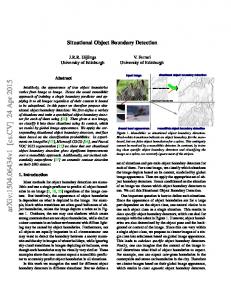
Equipped with location or range information (precisely, each node knows either its own location that may come with a certain error or the distances between itself and close-by nodes), geometric approaches often involve fairly localized computations and hence have the potential to be performed on-line. However, the discrete nature of a WSN “volume” may still make the local detection fairly complicated. On one hand, there is no commonly agreed definition for the boundary of a point cloud (the geometric representation of a WSN). For example, Figure 1 shows that whether a node

Figure 1: A node (white) and all its one-hop neighbors (black) are shown. Whether the white one is identified as on the boundary or not depends on the specific geometric interpretation. Precisely, the triangulation on the left indicates the node as on the boundary, but the answer is negative for the case on the right. The shaded ball is used to illustrate the idea of α-shape [4].

is at the boundary or not heavily depends on the specific geometric interpretation. On the other hand, the algorithms for boundary detection, albeit localized, can still incur a high time and/or message complexity. Zhang et al. [22] propose to use two local geometric structures, namely localized Voronoi polygon and neighbor embracing polygon, for boundary characterization only in 2D. It is shown in the paper that the detection procedure involves several rounds of interactions between (at least) all one-hop neighbors. Both [6] and [23] use a concept called α-shape [5] for boundary detection. In a nutshell, α-shape results from “erasing” the convex hull of a point cloud using a spherical “eraser” with a certain radius α: while 0-shape is the original point cloud, ∞-shape is the convex hull. In Figure 1, the left triangulation is actually an α-shape with α (roughly) equal to half of the transmission range. Although the α-shape construction leads to localized boundary detection, its computation cost is still non-negligible.

Remark :

Although we are concerned with boundary detection in 3D WSNs, we have to provide examples in 2D to facilitate visual illustration. However, our simulations will be performed for real 3D WSNs.

2.3

Event Boundary vs. Network Boundary

Some existing proposals tend to distinguish between event boundary and network boundary [23]. As we discussed in Sec. 1, we are concerned with both boundaries for the WSN applications under consideration. In fact, network boundary can be considered as a particular event boundary, with the “event” being the WSN itself. It is true that, whereas the network boundary is a clear-cut concept, other event boundaries can be rather fuzzy, due to sensing errors or smooth changes (in terms of certain physical quantities indicating the event) around the boundary. Fortunately, relying on statistic approaches such as [2], each node can arrive at a (binary) indicator on whether it covers a certain event or not. Therefore, making a distinction between these two types of boundaries may not be necessary.

2.4

Our Approach

In summary, a geometric approach that relies on the location or range information appears to be the right way towards a fast on-line boundary detection algorithm. The

demand of location/range information is not too much a constraint, given recent proposals for node localization in 3D WSNs (e.g., [14, 19]), as well as the fact that many events to be monitored are in open spaces and thus amenable to GPS localization. To cope with the notched boundaries (internal or external) of a 3D WSN, our approach is inspired by the principle that a transformed domain may offer features absent in the original domain. For example, a 3D (implicit) surface xyz = c is concave, but a logarithmic transformation makes it convex in the transformed domain: x0 +y 0 +z 0 = c0 with (·)0 = log(·). Therefore, the essence of our proposal is to find a simple transformation that “unfolds” the notched boundaries into convex ones, such that we can avoid the troublesome αshape construction and rely on a simple convexity test to locally detect boundary instead.

3.

UNFOLD: DETECTING BOUNDARY IN A “MIRROR” IMAGE

In this section, we first introduce our network model and give a brief overview of the basic ideas of UNFOLD. Then we describe the transformation used by UNFOLD to transform a point cloud (the geometric representation of a WSN), as well as our formal definitions of the boundaries for the point cloud. Finally, we present in detail the localized algorithm for boundary detection, along with its performance analysis. To maintain fluency, we postpone the proof details or sketches to the appendices.

3.1

UNFOLD in a Nutshell

We model a 3D WSN as a point cloud P = {pi |1 ≤ i ≤ n} ⊂ R3 , with each point pi representing a sensor node. We are not concerned with network topology, so the boundaries that we aim at detecting are purely geometric and only concern local network connectivity. We assume that each node has a convex transmission volume, such that a bi-directional communication link exists between this node and any other node within this volume. We denote by Ni the set of nodes within the transmission volume of node pi , or pi ’s one-hop neighbor set. We also assume that node pi is either aware of its geographic location or can measure the distance between itself and another node in Ni . As explained in Sec. 2.2, the difficulty of determining whether a node is on the boundary stems from the existence of notches and, more importantly, from the absence of convex boundary due to consecutive notches; one would need to rely on the fairly complicated α-shape construction to identify boundary nodes. Our UNFOLD applies a special transformation to “blow up” a boundary such that it becomes almost convex, and we define a boundary node based on its local convexity. We illustrate the idea by Figure 2. Note that a single transformation may only blow boundary within a limited range of directions, so a few transformations are needed to detect a complete boundary. Given such a transformation, the localized algorithm for UNFOLD to perform boundary detection becomes pretty straightforward. Each node periodically exchanges location or range information with its one-hop neighbors to construct a local coordinate system. Then the transformation is applied to the coordinates of all nodes in Ni ∪ {pi }, possibly from different directions. In the transformed domain, node pi performs convexity test to check if it is on or out of the

Figure 2: A transformation that “blows up” a boundary. The length of a certain arrow in the left figure shows the “force” applied to that part of the boundary. The darker nodes in the right figure are those being blown up to the new convex boundary.

convex hull of Ni , and it indicates itself as a boundary node if this test succeeds. Relevant questions we need to address are listed as follows: Q1 What are the properties of the boundaries resulting from UNFOLD? Q2 How many transformations need to be applied? Q3 What if the location/range information for individual nodes comes with errors? In the following, we present detailed principles and algorithms for UNFOLD, while addressing these questions.

3.2

Transformation and Boundary Definition

As we mentioned in Sec. 2.2, there is no commonly agreed definition for the boundary of a point cloud. Our definition is based on the assumption that a point cloud results from sampling a certain hypothetical 3D volume. Therefore, a point is on the boundary of the point cloud if it lies on the hypothetical surface of that volume. As such a surface is unknown, we borrow the idea of direct visibility from [10]: a surface (hence the points lying on it) is what we can see from a certain viewpoint. We first present a transformation that enables the recognition of points on such a surface, then we define boundary and its properties.

3.2.1

Definitions

Given any subset P 0 ⊆ P, we associate with P 0 a local coordinate system, and we place a viewpoint v that does not belong to the convex hull of P 0 at the origin and set a spherical “mirror ” centered at v with radius R. The transformation for a point pi ∈ P 0 is given by: pi (1) p˘i = f (pi ) = pi + 2(R − kpi k) kpi k where k · k can be any norm and we take Euclidean norm k · k2 in this paper. We illustrate the effect of this “spherical reflection” in Figure 3. Our definition of point cloud boundary is based on the transformation f (·). Definition 1. For any point pi ∈ P 0 ⊆ P, pi is said to be on the boundary of P 0 with respect to a common transformation f (·) (defined by vSand R) if Ni ⊆ P 0 and p˘i lies on the convex hull of f (Ni ) {v}. We refer to Figure 3 for the two extreme cases of P 0 = Ni and P 0 = P. Note that, as the definition concerns the

R

3.2.2

R v

involving only local convexity test, however, allows boundary detection for both internal and external boundaries of a point cloud from all directions.

pi

pi

Properties

First, it is straightforward to show that the boundary definitions preserve convexity, i.e.,

v

Proposition 2. If pi is on the convex hull of P 0 ⊆ P and Ni ⊆ P 0 , then pi is on the boundary of P 0 with respect to a certain transformation f (·). (a) Local effect

(b) Global effect

Figure 3: The effect of f (·) (defined by the viewpoint v and the “mirror” with radius R) on point clouds. For Ni of an arbitrary point pi , the transformation effectively “bends” the locally concave surface to a convex one in the transform domain (a). Given a point cloud P in (b) and let P 0 = P, its image f (P) in the transform domain is shown, along with part of the detectable boundary. As demonstrated by the two amplified one-hop neighborhoods, points on non-convex surfaces (of the original 2D area) are also detected as boundary points.

In other words, if a point is on a (internal or external) surface of the hypothetical volume represented by P and is “visible” (due to locally convexity) from some viewpoint, it will be recognized as a boundary node. Secondly, our definition assures that a node not on any hypothetical surface will not be recognized as a boundary node, i.e., Proposition 3. If pi is recognized as a boundary node for P 0 ⊆ P with respect to a certain transformation f (·), p0i ∈ Ni will not be recognized as a boundary node if v, pi , p0i are collinear.

image of Ni in the transform domain, it focuses only on the local property of a point cloud. Actually, we have another definition of boundary for which even the transformation is made local:

This safety property suggests that the transformation does not flip a point strictly behind a hypothetical surface out of that surface. The third property states how much impact the transformation can have on a notched surface to “blow it up”. We first define a quantity to measure to what extent a point is notched locally.

Definition 2. For any point pi ∈ P 0 ⊆ P, pi is said to be on the boundary of P 0 with respect to a particular transformation fpi (·) (defined by vpi and Rpi that dependSon pi ) if Ni ⊆ P 0 and p˘i lies on the convex hull of fpi (Ni ) {vpi }.

Definition 3. Given pi ∈ P and Ni , if pi lies within the convex hull, conv(Ni ), of Ni , we define the Depth of Notch (DoN) d of pi as the distance from pi to the nearest plane on conv(Ni ). We illustrate the definition of DoN in Figure 4(a), and we

While the latter definition allows the transformation to be adapted to local geometry (hence requires only local range information), the former definition (which requires location information) may have certain practical significance.3 In general, these two definitions, on one hand, are both amenable to the design of localized algorithm. On the other hand, the local properties stated in both definitions do have a global implication to some extent, according to the following result. Proposition 1. If pi is a boundary point of P according to either definition, there exists a nontrivial P 0 , i.e., Ni ⊂ P 0 ⊆ P, and a transformation f 0 (·), such that f 0 (pi ) lies 0 0 S on the convex hull of f (P ) {v 0 }. In particular, pi is an external boundary point of P, iff f 0 (pi ) lies on the convex S hull of f 0 (P) {v 0 }. The transformation f (·) shown in (1) is inspired by an inversion applied in a quite different context [10]. Katz et al. [10] applies this inversion to identify visible points on part of the external boundary of a point cloud, our extension 3 Taking the recent BP oil spill as an example. Should a WSN be deployed to monitor the spill coverage, a question some Miami tourism authority might ask would be: how far is the spill frontline towards Key West? This question effectively asks for a boundary detection based on a common viewpoint at Key West.

rj d pi

a1 a2

v

ri

rk R

(a) Depth of Notch in 3D

(b) Depth of Notch in 2D

Figure 4: The definition of Depth of Notch (DoN) is shown in 3D (a). However, to simplify the interpretation, we analyze the 2D case in (b), which can be considered as a projection of the 3D case on a certain plane.

show that, given f (·) (with certain v and R), a node can be “blown” to the convex hull only if its DoN is below a certain threshold. The proposition, illustrated by Figure 4(b), is stated and proven in 2D for the sake of simplicity, but it is readily extensible to 3D.

Proposition 4. For a given f (·), pi is recognized as a boundary node for P 0 ⊆ P iff its DoN d satisfies: d=

ri (rj sin α1 + rk sin α2 ) − rj rk sin(α1 + α2 ) q , rj2 + rk2 − 2rj rk cos(α1 + α2 ) (2R−r )(2R−r ) sin(α +α )

1 2 k . If α1 = α2 = where ri ≤ 2R − (2R−rj j) sin α1 +(2R−r k ) sin α2 α, rj = rk = r in particular, d ≤ 2R(1 − cos α).

Given a common viewpoint transformation (Definition 1), (ri , rj , rk ) and (α1 , α2 ) are fixed to each point, but R can be tuned to adapt to different requirement on compensating d. If a transformation is chosen for individual points (Definition 2), all the parameters of the transformation can be tuned. In 3D, the condition stated in (Definition 4) needs to be satisfied within all planes that pass through the line determined by v and pi . Finally, we answer Q2 raised in Sec. 3.1 by showing that, no matter which direction a hypothetical surface is facing, only a constant number of transformations are needed to recognize points on this surface. Proposition 5. If pi is on a hypothetical (internal or external) surface of P and it satisfies the DoN criterion, at most four transformations (hence four viewpoints) are needed to recognize pi as a boundary point.

2. Transformation: Having the coordinates for all nodes S in Ni {pi } with respect to a origin v (or vpi ), node pi applies the transformation given in (1) to these coordinates and obtains their images. This step involves only simple computations. 3. Convexity Test: Each node pi performs a convexity test to decide whether S or not its image S p˘i is on the convex hull of f (Ni ) {v} (or fpi (Ni ) {v}). A basic algorithm is shown in Algorithm 1. We use ~ x to Algorithm 1 CVX–TEST Input: f (Ni ), p˘i , a coord. system with v as the origin Output: Binary indicator boundary(˘ pi ) 1: for all distinct node pair m1 , m2 ∈ f (Ni ) do ;b=p ~i · ~n; 2: ~n ← (~ pi − m ~ 1 ) × (~ pi − m ~ 2 ); ~n ← k~~n nk 3: boundary(˘ pi ) ← true; 4: for all m ∈ f (Ni )\{m1 , m2 } do 5: if m ~ · ~n > b then 6: boundary(˘ pi ) ← false; break; 7: end if 8: end for 9: if boundary(˘ pi ) = true then 10: break; 11: end if 12: end for

In summary, our boundary definitions based on f (·) have the following three properties:

represent the vector form of a point x ˘. The idea is to try all possible planes determined by p˘i and another two points in f (Ni ) (lines 1–3), and to check S whether one of them is a supporting plane for f (N ) {v} (lines i S 4–8), i.e., if f (Ni ) {v} lies on one side of that plane.

1. Safety I: Points that are surely on some surface will be identified as boundary points. 2. Safety II: Points that are surely not on any surface will not be identified as boundary points.

To improve the efficiency, we apply the divide-andconquer strategy. Observe that, after each inner loop (lines 4–8), points in f (Ni ) can be totally ordered under ≥, according to their inner products with the normal ~n. Therefore, instead of arbitrarily choosing a (m1 , m2 ) pair, we replace only one of the current two points with what is ordered first in f (Ni ) (ties broken arbitrarily), such that the replaced point lies on the same side as v with respect to the new plane. In fact, no sorting is needed; the maximum point is naturally obtained at the end of each inner loop (lines 4–8). The algorithm terminates if neither points can be replaced: either because replacing either of them separates another from v or because the node ordered first in f (Ni ) lies on the current plane (i.e., the plane is a supporting plane). The algorithm returns boundary(pi ) = true if the current plane is a supporting plane and returns boundary(pi ) = false otherwise. We call this enhanced algorithm CVX–TEST–DC.

3. Tunable Liveness: Points on a non-convex surface can be identified with a small number of properly tuned transformations.

3.3

On-Line Boundary Detection Algorithm

Given the definitions of transformation and boundary, we are ready to present our UNFOLD for on-line boundary detection. UNFOLD involves mainly three steps for each node in a WSN: 1. Local Interactions: Each node pi exchanges location or range information with its neighbors in Ni to construct a local coordinate system. This step is trivial if the location information is available (through, for example, [14, 19]); otherwise a certain 3D embedding algorithm (e.g., [17]) is used to create the coordinate system using mutual distances. The origin of the coordinate system is the viewpoint v. (a) If the location information is available, we could afford to have a common viewpoint v (Definition 1), which can be required by certain applications (such as the BP oil spill example we gave in footnote 3). (b) Viewpoint vpi (Definition 2) specific to every pi can always be applied. This is preferred if only range information is available, as otherwise we have to perform a costly procedure to gradually construct a global coordinate system with local range information (e.g., [8]).

Note that the algorithm is conducted by individual nodes without the need for time synchronization. Therefore, UNFOLD is a localized algorithm requires only asynchronous operations; this makes UNFOLD extremely efficient.

3.4

Performance Analysis

We analyze the performance of UNFOLD on two aspects. We first look at the (time) complexity of UNFOLD, which also represents the energy efficiency of the algorithm. Then we show the robustness of UNFOLD against location or range errors.

3.4.1

Complexity Analysis

Our analysis on UNFOLD focuses on the transformation and convexity test steps, as the first step either has a negligible complexity if location information is available or otherwise involves well known procedures that are commonly applied in other proposals (e.g., [23]). Assuming η = |Ni |, the complexity of the transformation is obviously Θ(η), as weSbasically apply the transformation (1) to all nodes in Ni {pi }. The complexity of the basic convexity test, CVX–TEST, is also obvious: as the outer iteration has η(η − 1) loops and the inner iteration has η − 2 loops, the complexity is Θ(η 3 ). Consequently, the complexity (both average and worst-case) of UNFOLD with CVX–TEST is Θ(η 3 ). Although this is same as that of the αshape based boundary detection [23], the actually CPU time (hence energy consumption) of UNFOLD is actually much less (as shown in Sec. 5.2). The reason is simple: convexity test involves only vector operations (which are basically arithmetic instructions), whereas α-shape construction entails complicated operations/procedures such as square root and solving equation systems. Moreover, we may further reduce the complexity of UNFOLD by applying the enhanced convexity test: CVX–TEST–DC. Proposition 6. The average-case complexity of CVX–TEST–DC is O(η log η). This effectively reduces the average-case complexity of UNFOLD to O(η log η). Although the worst-case complexity is Θ(η 2 ), those worst cases happen very rarely according to our experience.

3.4.2

Error Analysis

Given the fact that the geometric boundary of a point cloud is not well defined, it is impossible to perform error analysis rigorously, as there is no ground truth to be compared with. One may be able to create a set of artificial “ground truth” boundary points in simulations, by deliberately sampling on the surface of the volume from which a point cloud is derived (which is the method that we will apply in Sec. 5.1 to evaluate the robustness of UNFOLD). However, unless those points are sampled extremely dense, there are still chances that certain “under the surface” points are detected as boundary points, regardless of which boundary detection mechanism is used. It is definitely unreasonable to categorize these points as detection errors, as they may well be on the surface of another volume that results in the same point cloud. Consequently, the error analysis we discuss here is rather qualitative. If location information is available to every node, the error can be characterized by a small ball with radius ε around the expected location of the node, where ε can be the mean square error resulting from certain localization mechanism (e.g., GPS). If only range information between neighboring nodes is available, the initial errors come from the given ranging technique. However, this error will eventually be translated into location errors through a 3D embedding algorithm (e.g., [17]). In either case, ε cannot be too large compared with the radius of conv(Ni ), as otherwise it could be corrected (thus reduced) based the local connectivity relations. Therefore, we may safely assume that ε is bounded by the radius of conv(Ni ). For a boundary node (based on our definitions), the location errors may either decrease or increase DoN, if we con-

sider a node pi on or out of its local convex hull conv(Ni ) as having a non-positive DoN. Apparently, a decreased DoN has no impact on boundary detection, whereas an increased DoN is somewhat compensated by our transformation, according to Proposition 4. For a non-boundary node, there are two cases: either it is very close to a boundary node or it indeed lies in the very interior of the point cloud. The former case, compared with a boundary node, is inversely affected by location errors. As the node is anyway close to a boundary node, a false positive does not really compromise boundary detection. The latter case can hardly be affected by location errors, given the boundedness of these errors. In summary, UNFOLD is very robust against location errors; we will demonstrate this in Sec. 5.1.

4.

DISCUSSIONS

We briefly discuss two related issues in this section. These are limitations of UNFOLD, as well as potential mechanisms that may work along with UNFOLD.

4.1

Limitations of UNFOLD

For extremely sparse WSNs (e.g., average neighbor set size below 10), it is possible that most of the nodes are detected as boundary nodes. The reason is that, as |Ni | is small, it is highly probable that pi is very close to conv(Ni ). In other words, the DoN of pi is small from some viewpoint. This is actually a common problem for localized detection mechanisms, as they are all not concerned with global topology. Compared with other localized detection mechanisms such as [6, 23], UNFOLD has one more leverage against this overdetection. As the transformation can be tuned to be more sensitive to DoN, we can somewhat avoid over-detection at a price of slightly losing nodes close to the real boundary. One possible future work is to combine certain local topological information to remove these over-detected nodes.

4.2

Companions of UNFOLD

One important companion of UNFOLD is a data collection mechanism to gather the boundary information towards human users, if a global boundary information is needed. The volume surface can be reconstructed in a centralized way based on the collected boundary information.4 For our current implementation, we are using a generic routing protocol for collecting boundary information, but we are working on routing mechanisms that are adapted to this specific data collection. Another potential companion we are considering is an in-network data aggregation scheme to avoid transmitting all the boundary information while still allowing full surface reconstruction at the user side [21]. UNFOLD, as a boundary detection mechanism, can also be used to support greedy (geographic) routing. Especially, as shown in [16], greedy routing can be applied even if location information is not available. The basic idea there is to generate virtual coordinates based on the awareness of the external boundary. However, it is well known that a greedy routing may fail due to local minima resulting from “holes” within a WSN, and this problem gets even serious in 3D WSNs [4]. In our (on-going) companion work, we propose 4 Although the surface reconstruction can be performed in a distributed manner (e.g., [23]), localized computing is not a cost-effective way for this purpose. As the boundary information needs anyway to be collected, the centralized surface reconstruction is both energy and time efficient.

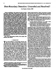
(a.1) 3691 nodes

(b.1) Top viewpoint: 912 boundary nodes

(c.1) 2607 boundary nodes

(a.2) 6795 nodes

(b.2) Left viewpoint: 640 boundary nodes

(c.2) 2560 boundary nodes

(a.3) 5902 nodes

(a.4) 10000 nodes

(a) Original networks

(b.3) Bottom viewpoint: 1230 boundary nodes

(b.4) Top viewpoint: 955 boundary nodes

(b) Boundary from a common viewpoint

(c.3) 4263 boundary nodes

(c.4) 3131 boundary nodes

(c) Boundary with local viewpoints

Figure 5: Boundary detection through UNFOLD. As the “shapes” of the WSNs may not be easily recognizable from their point clouds, we attach their original 3D volumes to respective point clouds (a). For boundary detection with a common viewpoint, boundary nodes are marked on top of the original clouds (b). We, however, remove the internal nodes when local viewpoints are applied to detecting the whole boundary (c). to combine UNFOLD (which detects both internal and external boundaries) with a greedy routing, in order to provide guaranteed delivery in 3D WSNs. The boundary information, along with a geographic routing protocol, can in turn serve as building blocks for constructing a distributed data management system in 3D WSNs [12, 13].

5.

SIMULATIONS AND EXPERIMENTS

We evaluate UNFOLD through both simulations and experiments. With simulations, we demonstrate the efficacy of UNFOLD in large scale WSNs. Through experiments based on an implementation in MICAz Motes, we confirm UNFOLD’s superiority in efficiency over the most up-to-date proposal [23].

5.1

Simulations

We first construct several 3D volumes to represent the physical events to be monitored. Then we randomly deploy sensor nodes in each volume and on the volume surface. As explained in Sec. 2.3, we may treat network and event boundary equivalently without loss of generality. Therefore, the goal of our simulations is to verify if UNFOLD can correctly identify the those points that we have deliberately put on the volume boundaries (which, according to Sec. 3.4.2, is an inevitable but artificial setting). Although UNFOLD applies to arbitrary convex transmission volumes, we assume a regular volume, a ball with radius r, for every node in order to simplify our presentation. We choose the value of r such that the average size of Ni is about 40.

# of Boundary Nodes

80% 70% 60% 50% 40% 30% 20%

90% 80% 70% 60% 50% 40% 30% 20% 10%

10% 0%

1−hop 2−hop

100%

0

r/6

r/3

r/2 2r/3 Error radius ε

5r/6

r

0%

100% Distribution of Missing Boundary Nodes

90%

Distribution of Mistaken Boundary Nodes

Found Correct Mistaken Missing

100%

90% 80% 70% 60% 50% 40% 30% 20% 1−hop 2−hop

10%

r/6

r/3

r/2 2r/3 Error radius ε

5r/6

r

0%

r/6

r/3

r/2 2r/3 Error radius ε

5r/6

r

(a) Algorithm efficiency

(b) Mistaken distribution

(c) Missing distribution

(d) ε = 16 r: 2554 boundary nodes

(e) ε = 13 r: 2189 boundary nodes

(f) ε = 32 r: 1902 boundary nodes

Figure 6: Boundary detection under location errors. We vary the error radius ε as different fractions of the transmission range r, and we both statistics (a–c) and an example (d–f ). The implementation of UNFOLD in our simulator follows the protocol description in Sec. 3.3. Specifically, each node first exchanges location information with its neighbors. As our high-level simulator neglects the MAC effect, this information exchange is considered to be reliable. In practice, the reliability can be achieved through, for example, ARQ. After collecting the neighbor information, all the computations left for a node are strictly localized: transformation and convexity test. In Figure 5, four examples of the simulated WSNs are shown. The WSNs, shown in the left column, are designed to exhibit various 3D shapes we may face in atmospheric or ocean monitoring. We apply UNFOLD with either common viewpoint or local viewpoints to perform boundary detection, and the results are shown in the central and right columns, respectively. It is clearly shown that, while a single common viewpoint only detects the boundaries that face the viewpoint, a few local viewpoints detect the whole boundary. Note that, though the inversion used in [10] only detects an external boundary, our extension also detects the internal boundary, as shown by the second and third WSNs. We also evaluate the robustness of UNFOLD under location errors. We assume each node has an error radius ε, such that the location information available to a node may be uniformly distributed within a ball with radius ε and centered at the real location. We then vary ε to different fractions of r, and apply UNFOLD to detect the boundary. In general, a node that is either a real boundary node or detected as a boundary node may have four states: • Found: detected as a boundary node • Correct: a boundary node and also detected as one • Mistaken: not a boundary node and detected as one • Missing: a boundary node and not detected as one

In Figure 6(a), we report the statistics in terms of these four states based on all the WSNs that we have simulated. We also report the statistics on the distance (in hop) from a mistaken/missing node to the closest correct boundary node in Figure 6(b) and (c). The same metrics are used in [23]; we reuse them to facilitate comparisons. As shown in Figure 6(a), both found and correct nodes decrease with an increasing error radius. However, even with the worst case error ε = r, correct nodes still account from around 50% the total boundary nodes. Also, the distributions in Figure 6(b) and (c) show that both mistaken and missing nodes are not far from the real boundary (at most two hops but mostly within one hop). We finally provide one example, corresponding the first WSN in Figure 5, in Figure 6(d–f). The message conveyed by all these figure is clear: although increasing location errors may marginally affect the detected boundaries (which is characterized by the found nodes), these boundaries still well characterizes the geometry of the network volume. Compared with the statistics reported in [23], UNFOLD appears to be more robust against the location errors: higher correct nodes percentage and shorter distances (from the mistaken and missing nodes) toward the real boundary.

5.2

Implementation and Experiments

We implement UNFOLD in MICAz Motes, and compare UNFOLD with the Unit Ball Fitting (UBF) algorithm proposed in [23] in terms of CPU time for boundary detection. Our experiments focus only on local computation steps, as the local communications to exchange location/range information are common to both approaches. Consequently, we use the location information sampled from our simulated WSNs and inject these data to a MICAz Mote, such that we can directly start the actually boundary identification steps: transformation/convexity tests for UNFOLD, and ball tests for UBF. As the microcontroller of our MICAz (ATMEL AT-

Mega 128L) is fully occupied (i.e., never in idle mode or being interrupted) during both computations, we may roughly use the CPU time to also represent the energy consumption spent for computations. Consequently, our experiments also compare UNFOLD with UBF in terms of energy efficiency. We show two sets of results, internal and boundary nodes, in Figure 7 and 8, respectively. The comparisons are made between UBF and two versions of UNFOLD that differ in the convexity test algorithms. As an internal node is often the worst case for all the three schemes, Figure 7 serves as a confirmation of the complexity analysis (Sec. 3.4.1). Because the complexity of both UBF and CVX–TEST are Θ(η 3 ), the more than 10 times difference between them stems from the simple computations incurred by CVX–TEST. Another more than 10 times improvement brought by CVX–TEST– DC follows from its O(η log η) complexity. UBF CVX−TEST CVX−TEST−DC

4

CPU time (ms)

10

UBF. In fact, with a CPU time of tens of seconds, UBF may not even be eligible for an on-line boundary detection.

6.

CONCLUSION

We have investigated the challenging problem of on-line boundary detection in 3D WSNs, and we have proposed UNFOLD as a concrete solution to this problem. UNFOLD significantly speeds up the boundary detection by performing it in a transformed domain. This makes it perfectly suitable for on-line boundary detection in 3D WSNs that are deployed for monitoring time-variant physical events. We have demonstrated the efficiency and efficacy of UNFOLD through both simulations and experiments (using a MICAzbased testbed). Compared with an up-to-date proposal, UNFOLD is, on one hand, more robust against the location errors, and on the other hand, UNFOLD is far more efficient in terms of both computation time and energy consumption. Our future work, apart from the companions discussed in Sec. 4.2, involves the development of a full-fledged testbed for comparing various boundary detection schemes.

7.

ACKNOWLEDGEMENTS

We are grateful to the anonymous reviewers and our shepherd Lakshmi Subramanian for their constructive feedback.

3

10

8.

REFERENCES

2

10

20

30

40

50

60

70

80

90

# of node in the neighbor set Ni

Figure 7: CPU times for internal nodes.

UBF CVX−TEST CVX−TEST−DC

4

CPU time (ms)

10

3

10

2

10

36

38

40

42

44

46

48

50

52

54

56

# of node in the neighbor set Ni

Figure 8: CPU times for boundary nodes.

For boundary nodes (Figure 8), all the three schemes may face cases varying from the best to the worst. Therefore, the CPU times are rather dispersed, but the roughly 100-time advantage of CVX–TEST–DC over UBF still holds. Note that the fairly constant (and almost always the smallest) CPU times for CVX–TEST–DC mostly indicate the cost of the transformation f (Ni ). In summary, UNFOLD with CVX–TEST–DC is far more time and energy efficient than

[1] T.H. Cormen, C.E. Leiserson, R.L. Rivest, and C. Stein. Introduction to Algorithms. MIT Press, Cambridge, MA, 2 edition, 2001. [2] M. Ding, D. Chen, K. Xing, and X. Cheng. Localized Fault-Tolerant Event Boundary Detection in Sensor Networks. In Proc. of the 24th IEEE INFOCOM, 2005. [3] D. Dong, Y. Liu, and X. Liao. Fine-Grained Boundary Recognition in Wireless Ad Hoc and Sensor Networks by Topological Methods. In Proc. of the 10th ACM MobiHoc, 2009. [4] S. Durocher, D. Kirkpatrick, and L. Narayanan. Guaranteed Delivery in Three-Dimensional Ad Hoc Wireless Networks. In Proc. of the 9th ICDCN, 2008. [5] H. Edelsbrunner, D. Kirkpatrick, and R. Seidel. On the Shape of a Set of Points in the Plane. IEEE Trans. on Information Theory, 29(4):551–559, 1983. [6] M. Fayed and H. Mouftah. Localised Alpha-Shape Computations for Boundary Recognition in Sensor Networks. Elsevier Ad Hoc Networks, 7(6):1259–1269, 2009. [7] R. Ghrist and A. Muhammad. Coverage and Hole-Detection in Sensor Networks via Homology. In Proc. of the 4th ACM/IEEE IPSN, 2005. [8] D. Goldenberg, P. Bihler, M. Cao, J. Fang, B. Anderson, A.S. Morse, and Y.R. Yang. Localization in Sparse Networks using Sweeps. In Proc. of the 12th ACM MobiCom, 2006. [9] B. Joe. Three-Dimensional Triangulations from Local Transformations. SIAM J. Sci. Stat. Comput., 10(4):718–741, 1989. [10] S. Katz, A. Tal, and R. Basri. Direct Visibility of Point Sets. In Proc. of the 34th ACM SIGGRAPH, 2007. [11] A. Kr¨ oller, S. Fekete, D. Pfisterer, and S. Fischer. Deterministic Boundary Recognition and Topology

[12]

[13]

[14]

[15]

[16]

[17]

[18]

[19]

[20]

[21]

[22]

[23]

Extraction for Large Sensor Networks. In Proc. of the 17th ACM/SIAM SODA, 2006. J. Luo and Y. He. GeoQuorum: Load Balancing and Energy Efficient Data Access in Wireless Sensor Networks. In Proc. of the 30th IEEE INFOCOM (mini-conference), 2011. J. Luo, F. Li, and Y. He. 3DQS: Distributed Data Access in 3D Wireless Sensor Networks. In Proc. of the IEEE ICC, 2011. J. Luo, H.V. Shukla, and J.-P. Hubaux. Non-Interactive Location Surveying for Sensor Networks with Mobility-Differentiated ToA. In Proc. of the 25th IEEE INFOCOM, 2006. R. Nowak and U. Mitra. Boundary Estimation in Sensor Networks. In Proc. of the 2nd ACM/IEEE IPSN, 2003. A. Rao, S. Ratnasamy, C. Papadimitriou, S. Shenker, and I. Stoica. Geographic Routing without Location Informtion. In Proc. of the 9th ACM MobiCom, 2003. Y. Shang and W. Ruml. Improved MDS-Based Localization. In Proc. of the 23rd IEEE INFOCOM, 2004. S. Subramanian, S. Shakkottai, and P. Gupta. Optimal Geographic Routing for Wireless Networks with Near-arbitrary Holes and Traffic. In Proc. of the 27th IEEE INFOCOM, 2008. G. Tan, H. Jiang, S. Zhang, and A.-M. Kermarrec. Connectivity-based and Anchor-Free Localization in Large-Scale 2D/3D Sensor Networks. In Proc. of the 11th ACM MobiHoc, 2010. Y. Wang, J. Gao, and J. Mitchell. Boundary Recognition in Sensor Networks by Topological Methods. In Proc. of the 12th ACM MobiCom, 2006. L. Xiang, J. Luo, and A. Vasilakos. Compressed Data Aggregation for Energy Efficient Wireless Sensor Networks. In Proc. of the 8th IEEE SECON (to appear), 2011. C. Zhang, Y. Zhang, and Y. Fang. Localized Algorithms for Coverage Boundary Detection in Wireless Sensor Networks. Springer Wireless Networks, 15(1):3–20, 2009. H. Zhou, S. Xia, M. Jin, and H. Wu. Localized Algorithm for Precise Boundary Detection in 3D Wireless Networks. In Proc. of the 30th IEEE ICDCS, 2010.

APPENDIX We hereby provide (detailed or sketched) proofs for the propositions stated in our paper.

A.

PROOFS OF PROPOSITION 1

Let pi be on the boundary of P according to either Definition 1 or 2, and let v be the concerned viewpoint. Without loss of generality, we may expand Ni to a nontrivial P 0 ⊆ P such thatSNi ⊂ P 0 , simply by adding one more point, i.e., P 0 = Ni {p0 }. There are two possible cases: p0 lies either on or not on the line segment between v and pi . As p0 6∈ conv(Ni ) (otherwise we would have p0 ∈ Ni , given the convexity of the transmission volume), we can avoid the former case by choosing v very close to the boundary of conv(Ni ). For the latter case, we simply let v 0 = v. Ac-

cording to the “blowing-up” feature of the transformation f (·) (which will be quantified by Proposition 4), there al0 0 ways exists S an f (·) such that f (pi ) lies on the convex hull of f 0 (P 0 ) {v 0 }, as far as there is no point in P 0 that lies on the line segment between v 0 and pi . In particular, if pi is on the external boundary of P, it is “visible” from some viewpoint v 0 . Therefore, we can directly expand Ni to P and be sure that no p0 ∈ P is on the line segment between v 0 and pi . Consequently, there exists S an f 0 (·) such that f 0 (pi ) lies on the convex hull of f 0 (P) {v 0 }. Conversely, the existenceSof an f 0 (·) such that f 0 (pi ) lies on the convex hull of f 0 (P) {v 0 } suggests that no p0 ∈ P is on the line segment between v 0 and pi . Since v 0 6∈ conv(P), pi has to be on the external boundary of P. Q.E.D.

B.

PROOFS OF PROPOSITIONS 2 AND 3

It is straightforward to verify that the transformation f (·) preserves surface convexity. In other words, if part of the surface is described by a convex function, this convexity is preserved in the image of f (·). The fact that pi is on the convex hull of P 0 ⊆ P suggest that the surface through pi is locally convex. Therefore, simply choosing a viewpoint v that faces that surface and applying a proper f (·) will lead to the claim made in Proposition 2. Based on the formulation of f (·), it is trivial to show that, if v, pi , p0i are collinear, then v, pi , p0i , f (pi ), f (p0i ) are also collinear. Therefore, at most one of pi and p0i can be recognized as a boundary node, hence the claim made in Proposition 3 follows. Q.E.D.

C.

PROOFS OF PROPOSITIONS 4 AND 5

We only sketch the proof of Proposition 4 by omitting the tedious trigonometric derivations. To derive the upper bound for d, we consider the worst case where the images of the three points become collinear, as shown in Figure 9(a), because further increasing d would compromise the convexity of p˘i . Using basic trigonometry, we can obtain the relation between d and (ri , rj , rk , α1 , α2 ) as d=

ri (rj sin α1 + rk sin α2 ) − rj rk sin(α1 + α2 ) q . rj2 + rk2 − 2rj rk cos(α1 + α2 )

Obviously, given (rj , rk , α1 , α2 ), d is increasing in ri . Therefore, we bound d from above by bounding ri . The key to subsequent derivations is: β1 + β2 = π ⇒ tan β1 + tan β2 = 0 in the worst case shown in Figure 9(a). Using (R, rj , rk , α1 , α2 ) to represent tan β1 and tan β2 , we have ri ≤ 2R −

(2R − rj )(2R − rk ) sin(α1 + α2 ) . (2R − rj ) sin α1 + (2R − rk ) sin α2

The case where α1 = α2 and rj = rk follows trivially. The statement that four transformations are sufficient to recognize boundary points follows from the sufficiency of “seeing” a whole spherical surface from four viewpoints. If pi is on a hypothetical surface of P, we need a viewpoint v from which this surface is visible. As our convexity test is localized, all the surfaces of conv(Ni ) need to be tested, we hence need a sufficient number of viewpoints for all these surfaces. As we can embed the surface of conv(Ni ) in the surface of an enclosing ball Bi centered at pi , the visibility of conv(Ni ) is equivalent to that of Bi . We put a tetrahedron Ti with vertices v1 , v2 , v3 , v4 that encloses Bi , as shown in Figure 9(b). For any point p on

v2 rj

pj

b1 d pi p r b2 i pk i

a1 a2

v rk

p v1

pi

Bi

v3

R v4 (a) Depth of Notch

(b) Visibility of ball surface

Figure 9: Illustrations for proofs. (a) Depth of Notch (DoN) in 2D – the extreme case, and (b) the ball surface is visible from at least one vertex of an enclosing tetrahedron.

the surface of Bi , the condition that it is not visible from any vertex is that (~ p−p ~i ) · (~vj − p ~) < 0, ∀j = 1, 2, 3, 4. However, as p, along with the three closest vertices (v1 , v2 , v4 in Figure 9(b) for example), form another tetrahedron Tp , the condition for invisibility contradicts the fact that p ~−p ~i points to the interior of Tp from point p. Therefore, our claim in Proposition 5 follows. Q.E.D.

D.

As f (Ni ) is a finite set, Lemma 1 shows that CVX–TEST– DC terminates in finite time regardless of the status of p˘i . If S p˘i is on the convex hull of f (Ni ) {v}, the correctness of the algorithm is obvious. Otherwise the correctness is confirmed by the following result. Lemma 2. If neither mk−1 nor mk can be replaced at the k-th iteration and the current plane is not S a supporting plane, p˘i is not on the convex hull of f (Ni ) {v}. Proof. Let us consider the simplex induced by the set {v, mk−1 , mk , mk+1 } in Figure 10(b), where mk+1 is a candidate to be added for the next iteration. The assumption that mk+1 cannot replace either mk−1 or mk implies that a plane determined by p˘i and any two points in {mk−1 , mk , mk+1 } separates the third from v. It is straightforward to show that this is possible only if p˘i is inside the simplex, hence S proving p˘i is not on the convex hull of f (Ni ) {v}.

m

k

mk-1 pi v

m

k+1

PROOF OF PROPOSITION 6

For the k-th outer iteration, let ~nk and ~nk · p ~i denote the plane used for the test, i.e., ~nk · m ~ = ~nk ·~ pi , ∀m ∈ R3 , and let ˘ik be the subset of f (Ni ) that belongs to the convex hull N of {v, m1 , · · · , mk , p˘i }, where mk refers to the point chosen ˘ik } is a strictly for the k-th iteration. We first show that {N increasing sequence. ˘ik ⊂ N ˘ k+1 . Lemma 1. N i ˘ik ⊆ Proof. Given the construction, it is clear that N k+1 k+1 k ˘ ˘ ˘ Ni . Assume, by contradiction, that Ni = Ni . This ˘ik , and hence contradicts the fact implies that mk+1 ∈ N k+1 that m ~ is the largest among f (Ni ) in terms of its inner product with ~nk .

Figure 10: Illustration for proof of Lemma 2. It is straightforward to see that CVX–TEST–DC is similar to quicksort, as the new point chosen in each iteration acts in a similar way as the pivot in quicksort. Moreover, CVX– ˘ik after TEST–DC only needs to “conquer” points in Ni \N dividing. Therefore, we have the following recurrence for the time complexity T (η), given totally η points in f (Ni ): T (η) = T (cη) + O(η),

0 < c < 1,

According to master theorem [1], the average-case complexity of CVX–TEST–DC is O(η log η). Q.E.D. It can be shown that the average-case of complexity of CVX–TEST–DC in 2D is only O(log η), demonstrating again the non-trivialness of extending from 2D to 3D.