Fast Ideal Arithmetic in Quadratic Fields - Semantic Scholar

THE UNIVERSITY OF CALGARY

Fast Ideal Arithmetic in Quadratic Fields

by

Reginald Sawilla

A THESIS SUBMITTED TO THE FACULTY OF GRADUATE STUDIES IN PARTIAL FULFILLMENT OF THE REQUIREMENTS FOR THE CROSS-DISCIPLINARY DEGREE OF MASTER OF SCIENCE

DEPARTMENT OF MATHEMATICS AND STATISTICS and DEPARTMENT OF COMPUTER SCIENCE

CALGARY, ALBERTA AUGUST, 2004

c Reginald Sawilla 2004

THE UNIVERSITY OF CALGARY FACULTY OF GRADUATE STUDIES

The undersigned certify that they have read, and recommend to the Faculty of Graduate Studies for acceptance, a thesis entitled “Fast Ideal Arithmetic in Quadratic Fields” submitted by Reginald Sawilla in partial fulfillment of the requirements for the degree of CROSS-DISCIPLINARY DEGREE OF MASTER OF SCIENCE.

Chair, Supervisor, Dr. H.C. Williams Department of Mathematics and Statistics

Co-Supervisor, Dr. M.J. Jacobson Department of Computer Science

Dr. M.L. Bauer Department of Mathematics and Statistics

Dr. R. Scheidler Department of Computer Science

Dr. B.H. Far Department of Electrical and Computer Engineering

Date ii

Abstract Ideal multiplication and reduction are fundamental operations on ideals and are used extensively in class group and infrastructure computations; hence, the efficiency of these operations is extremely important. In this thesis we focus on reduction in real quadratic fields and examine all of the known reduction algorithms, converting them whenever required to work with ideals of positive discriminant. We begin with the classical algorithms of Gauss and Lagrange and move on to the algorithm Rickert developed for the closely related case of positive definite binary quadratic forms. Given any reduction technique, we present a general method computing the relative generator necessary for infrastructure computations. Rickert’s algorithm along with an algorithm of Schönhage are adapted to ideals of real quadratic fields. We present a new method which combines the ideas of Lehmer, Williams, and others into a particularly simple algorithm. All of these algorithms have been implemented and compared with the Jacobson-Scheidler-Williams adaptation of NUCOMP in a cryptographic public key-exchange protocol. We conclude showing that Schönhage’s algorithm is asymptotically the fastest but not useful in practice, JSW-NUCOMP is the fastest practical method when multiplying and reducing, and the new algorithm is the fastest method when only reduction is required.

iii

Acknowledgments I would like to thank my supervisor, Dr. Hugh Williams, for his invaluable advice, both professional and scholarly. His tireless work in establishing the Centre for Information Security and Cryptography (CISaC) has developed a fertile research environment among the best anywhere. This environment and the opportunity to study under his tutelage are the primary reasons I chose the University of Calgary. I also thank my co-supervisor, Dr. Michael Jacobson. His friendly encouragement and patient help have been greatly appreciated on many occasions. The camaraderie we have shared has contributed significantly to the enjoyment of this experience. I thank both of my supervisors for their excellence and the huge role they have played in the development of this thesis. Thank you to the other members of my examining committee, Dr. Mark Bauer, Dr. Renate Scheidler and Dr. Behrouz Far. The time and effort you have spent reading the thesis and giving advice is greatly appreciated. I would like to especially thank Dr. Scheidler who has put up with more of me than duty requires due to her close proximity to my office. I have so appreciated my fellow students for their practical help with academic questions, patience in listening to my talks, and for their friendship. I have thoroughly

iv

enjoyed the good times, food and games we have shared and have learned many things about myself, Calgary and other countries and cultures through them. I would like to thank Dr. Amir Akbary at the University of Lethbridge for introducing me to number theory and cryptography. In two summer research sessions he generously gave me the freedom to pick any mathematical topic of study and pursue any angle of research that interested me. He liberally gave of his time and resources and was a significant factor in my decision to pursue graduate studies. I am grateful to NSERC, iCORE, Dr. Williams, Dr. Scheidler and the University of Calgary for the funding provided to make this degree possible. The funding has taken many forms including research stipends, funds to attend conferences and workshops, and provision of computer equipment, all of which has enriched the academic experience. I especially thank my wife Darcie who has been so supportive throughout my education. Similarly, I am indebted to each of my children Shafir, Aliya, Ciara, and Eve who have all made sacrifices. Most of all I am grateful to God for his guidance, wisdom and favour. Apart from Him, I can do nothing.

v

Dedication I dedicate this thesis to: My father: Though his time on earth was cut short, his influence upon me has been profound. My mother: To whom I am forever indebted for her endless encouragement, support and prayers. My wife: The most important person in my life and best friend.

vi

Contents Approval Page

ii

Abstract

iii

Acknowledgments

iv

Dedication

vi

Contents

vii

List of Tables

ix

List of Figures

x

List of Algorithms

xi

Frequently Used Notation

xii

1 Introduction 1.1 Ideal Arithmetic . . . . . . . . . . . . . . . . . . . . . . . . . . . . . . 1.2 Organization Of The Thesis . . . . . . . . . . . . . . . . . . . . . . .

1 1 4

2 Algebraic Number Theory Concepts 2.1 Algebraic Number Fields . . . . . . . . . . . . . . . . . . . . . . . . . 2.2 Ideals . . . . . . . . . . . . . . . . . . . . . . . . . . . . . . . . . . . 2.3 Class Group and Class Number . . . . . . . . . . . . . . . . . . . . .

6 6 14 18

3 Multiplication and Reduction 3.1 Multiplication . . . . . . . . 3.2 Equivalence . . . . . . . . . 3.2.1 Equivalence Classes . 3.2.2 Relative Generator .

24 25 26 26 31

Theory . . . . . . . . . . . . . . . . . . . . vii

. . . .

. . . .

. . . .

. . . .

. . . .

. . . .

. . . .

. . . .

. . . .

. . . .

. . . .

. . . .

. . . .

. . . .

. . . .

. . . .

. . . .

. . . .

3.3

3.4 3.5

Reduction . . . . . . . . . . . . . . 3.3.1 Purpose of Reduction . . . . 3.3.2 Classical Reduction of Ideals Finding a Reduced Representative . Binary Quadratic Forms . . . . . .

. . . . . . . . . . . . . . (Lagrange) . . . . . . . . . . . . . .

. . . . .

. . . . .

. . . . .

. . . . .

. . . . .

. . . . .

. . . . .

. . . . .

. . . . .

. . . . .

. . . . .

. . . . .

34 34 34 41 42

4 Applications to Secure Communication

51

5 Survey of Improved Algorithms 5.1 Rickert’s Algorithm . . . . . . . . . . . 5.2 Schönhage’s Algorithm . . . . . . . . . 5.3 Schnorr and Seysen’s Algorithm . . . . 5.4 A New Algorithm For Ideal Reduction 5.5 Shanks’ Algorithm – NUCOMP . . . . 5.6 Improvements to NUCOMP . . . . . . 5.7 Complexity . . . . . . . . . . . . . . .

. . . . . . .

. . . . . . .

. . . . . . .

. . . . . . .

. . . . . . .

. . . . . . .

. . . . . . .

. . . . . . .

. . . . . . .

. . . . . . .

. . . . . . .

. . . . . . .

. . . . . . .

. . . . . . .

. . . . . . .

. . . . . . .

. . . . . . .

57 58 63 73 78 84 87 92

6 Implementation and Timings 6.1 General Principles . . . . . . . . . . . . 6.2 Lehmer’s Extended GCD Algorithm . . 6.3 Rickert’s Algorithm . . . . . . . . . . . 6.4 Schönhage’s Algorithm . . . . . . . . . 6.5 A New Algorithm For Ideal Reduction 6.6 Jacobson-Scheidler-Williams NUCOMP 6.7 Timings . . . . . . . . . . . . . . . . .

. . . . . . .

. . . . . . .

. . . . . . .

. . . . . . .

. . . . . . .

. . . . . . .

. . . . . . .

. . . . . . .

. . . . . . .

. . . . . . .

. . . . . . .

. . . . . . .

. . . . . . .

. . . . . . .

. . . . . . .

. . . . . . .

. . . . . . .

95 95 98 101 103 107 109 112

7 Conclusion

119

Bibliography

122

A An Improved Composition Algorithm

129

viii

List of Tables 5.1

Known Reduction Algorithm Complexity Results . . . . . . . . . . .

6.1 Calculation of Qi , Pi and Ri . . . . . . . . . . . 6.2 Average Key Exchange Times In Seconds . . . . 6.3 Single Key Exchange Times In Seconds . . . . . 6.4 Estimating Functions For Key Exchange Times

ix

. . . .

. . . .

. . . .

. . . .

. . . .

. . . .

. . . .

. . . .

. . . .

. . . .

. . . .

. . . .

94 109 114 115 117

List of Figures 4.1

Message And Key Transmission . . . . . . . . . . . . . . . . . . . . .

52

5.1

Magic Matrix . . . . . . . . . . . . . . . . . . . . . . . . . . . . . . .

85

6.1 6.2

Key Exchange Comparison . . . . . . . . . . . . . . . . . . . . . . . . 115 Key Exchange Comparison (Logarithmic) . . . . . . . . . . . . . . . . 116

x

List of Algorithms 3.1 Rho(ρ) — one continued fraction expansion step 3.2 Continued Fraction Reduction (Matrix) . . . . . 3.3 Continued Fraction Reduction (Ideal) . . . . . . 3.4 Continued Fraction Reduction (Implementation) 3.5 Near Reduced Ideal (Ideal) . . . . . . . . . . . . 3.6 Gaussian Reduction (Matrix) . . . . . . . . . . 3.7 Gaussian Reduction (Ideal) . . . . . . . . . . . 3.8 Gaussian Reduction (Implementation) . . . . .

. . . . . . . .

. . . . . . . .

. . . . . . . .

. . . . . . . .

. . . . . . . .

. . . . . . . .

. . . . . . . .

. . . . . . . .

. . . . . . . .

. . . . . . . .

. . . . . . . .

. . . . . . . .

36 37 38 39 42 48 49 50

5.1 5.2 5.3 5.4 5.5 5.6 5.7 5.8 5.9 5.10

Rickert–Style Reduction Algorithm (Matrix) . . Rickert–Style Reduction Algorithm (Ideal) . . . Schönhage Reduction (Matrix) . . . . . . . . . . Make Positive (Matrix) . . . . . . . . . . . . . . Monotone Reduction — MR (Matrix) . . . . . . Simple Step Above 2m (Matrix) . . . . . . . . . Simple Step Above 2m (Ideal) . . . . . . . . . . Efficient Ideal Reduction (Ideal) . . . . . . . . . Efficient Ideal Reduction (Matrix) . . . . . . . . Jacobson-Scheidler-Williams NUCOMP (Basic)

. . . . . . . . . .

. . . . . . . . . .

. . . . . . . . . .

. . . . . . . . . .

. . . . . . . . . .

. . . . . . . . . .

. . . . . . . . . .

. . . . . . . . . .

. . . . . . . . . .

. . . . . . . . . .

. . . . . . . . . .

. . . . . . . . . .

61 62 64 65 66 71 72 82 83 93

6.1 6.2 6.3 6.4 6.5 6.6 6.7 6.8

Lehmer’s Extended GCD (with Jebelean’s condition) . . . Rickert–Style Reduction Algorithm (Implementation) . . . Schönhage Reduction (Implementation) . . . . . . . . . . . Make Positive (Implementation) . . . . . . . . . . . . . . . Monotone Reduction — MR (Implementation) . . . . . . . Simple Step Above 2m (Implementation) . . . . . . . . . . Efficient Ideal Reduction (Implementation) . . . . . . . . . Jacobson-Scheidler-Williams NUCOMP (Implementation) .

. . . . . . . .

. . . . . . . .

. . . . . . . .

. . . . . . . .

. . . . . . . .

. . . . . . . .

100 102 103 104 105 106 108 111

xi

Frequently Used Notation General ≈

Approximately equal to . . . . . . . . . . . . . . . . . . . . . . . . . . . . . . . . . . . . . . . 23

∈

Is an element of . . . . . . . . . . . . . . . . . . . . . . . . . . . . . . . . . . . . . . . . . . . . . . . . 7

⊆ P

Subset or subring . . . . . . . . . . . . . . . . . . . . . . . . . . . . . . . . . . . . . . . . . . . . . . 7

Q

Product . . . . . . . . . . . . . . . . . . . . . . . . . . . . . . . . . . . . . . . . . . . . . . . . . . . . . . . 61

dae

Ceiling of a . . . . . . . . . . . . . . . . . . . . . . . . . . . . . . . . . . . . . . . . . . . . . . . . . . . 61

bac

Floor of a . . . . . . . . . . . . . . . . . . . . . . . . . . . . . . . . . . . . . . . . . . . . . . . . . . . . . 23

a ˆ

Single-precision approximation of a. . . . . . . . . . . . . . . . . . . . . . . . . . . . 58

|a|

Absolute value of a . . . . . . . . . . . . . . . . . . . . . . . . . . . . . . . . . . . . . . . . . . . 23

(a, b, c)

Binary quadratic form . . . . . . . . . . . . . . . . . . . . . . . . . . . . . . . . . . . . . . . . 43

Summation . . . . . . . . . . . . . . . . . . . . . . . . . . . . . . . . . . . . . . . . . . . . . . . . . . . 15

[q0 , . . . , qn−1 , αn ] Simple continued fraction expansion . . . . . . . . . . . . . . . . . . . . . . . . . . . 35 det M Qi Pi Pi Ri

Determinant of the matrix M . . . . . . . . . . . . . . . . . . . . . . . . . . . . . . . . . 29

A matrix . . . . . . . . . . . . . . . . . . . . . . . . . . . . . . . . . . . . . . . . . . . . . . . . . . . . . . 26

{ai |T }

Set comprised of elements ai subject to condition T . . . . . . . . . . . 15

a←b

Set a to the value of b . . . . . . . . . . . . . . . . . . . . . . . . . . . . . . . . . . . . . . . . . 36

Ai , Bi

Sequences from a simple continued fraction expansion . . . . . . . . . 35

c|a

c divides a . . . . . . . . . . . . . . . . . . . . . . . . . . . . . . . . . . . . . . . . . . . . . . . . . . . . 21

xii

I2

2 × 2 identity matrix . . . . . . . . . . . . . . . . . . . . . . . . . . . . . . . . . . . . . . . . . . 27

C

Field of complex numbers . . . . . . . . . . . . . . . . . . . . . . . . . . . . . . . . . . . . . . 7

Q

Field of rational numbers . . . . . . . . . . . . . . . . . . . . . . . . . . . . . . . . . . . . . . . 7

Z

Ring of rational integers . . . . . . . . . . . . . . . . . . . . . . . . . . . . . . . . . . . . . . . . 8

gcd

Greatest common divisor . . . . . . . . . . . . . . . . . . . . . . . . . . . . . . . . . . . . . . 25

Functions λM

Function representing the action of the matrix M on a quadratic irrational . . . . . . . . . . . . . . . . . . . . . . . . . . . . . . . . . . . . . . . . . . . . . . . . . . . . . 28

φN

Function representing the action of the matrix N on a 2 × 2 matrix . . . . . . . . . . . . . . . . . . . . . . . . . . . . . . . . . . . . . . . . . . . . . . . . . . . . . . . . . . 29

f :A→B

A function f mapping from A into B . . . . . . . . . . . . . . . . . . . . . . . . . . 12

a 7→ b

Element a maps to the element b . . . . . . . . . . . . . . . . . . . . . . . . . . . . . . 29

f (α)

Polynomial f evaluated at α . . . . . . . . . . . . . . . . . . . . . . . . . . . . . . . . . . . 7

f (n) = O(g(n)) Big-O, f (n) ≤ cg(n) for some constant c when n is sufficiently large . . . . . . . . . . . . . . . . . . . . . . . . . . . . . . . . . . . . . . . . . . . . . . . . . . . . . . . . . 34

Groups, Rings and Fields [E : F ]

Degree of E over F . . . . . . . . . . . . . . . . . . . . . . . . . . . . . . . . . . . . . . . . . . . . 7

α ¯

Conjugate of the quadratic irrational element α . . . . . . . . . . . . . . . 14

∆K

Discriminant of the number field K . . . . . . . . . . . . . . . . . . . . . . . . . . . 12

OK

Ring of integers of the number field K . . . . . . . . . . . . . . . . . . . . . . . . . . 9

PGL(2, Z) √ Q( D)

The factor group GL(2, Z)/ ± I2 . . . . . . . . . . . . . . . . . . . . . . . . . . . . . . . 27 Quadratic number field and D is a square-free integer . . . . . . . . . 12

{α1 , α2 , . . . , αn } Set or basis . . . . . . . . . . . . . . . . . . . . . . . . . . . . . . . . . . . . . . . . . . . . . . . . . . . 11 F (α)

Extension field formed by adjoining α to F . . . . . . . . . . . . . . . . . . . . . 7

K

An algebraic number field . . . . . . . . . . . . . . . . . . . . . . . . . . . . . . . . . . . . . . 8 xiii

Ideals σ

σ = 2 if D ≡ 1 (mod 4), and σ = 1 otherwise . . . . . . . . . . . . . . . . . . 13

ab

Ideal a multiplied by ideal b. . . . . . . . . . . . . . . . . . . . . . . . . . . . . . . . . . . 15

a∼b

Ideal a is equivalent to ideal b . . . . . . . . . . . . . . . . . . . . . . . . . . . . . . . . . 19

[a]

Equivalence class of the ideal a . . . . . . . . . . . . . . . . . . . . . . . . . . . . . . . . 19

aZ ⊕ bZ

Z-module . . . . . . . . . . . . . . . . . . . . . . . . . . . . . . . . . . . . . . . . . . . . . . . . . . . . . 21

N (a) (Q, P )

Norm of the ideal a . . . . . . . . . . . . . . . . . . . . . . . . . . . . . . . . . . . . . . . . . . . 21 √ Ideal generated by Q/σ and (P + D)/σ . . . . . . . . . . . . . . . . . . . . . 22

Ai

Matrix corresponding to the ideal (Qi , Pi ) . . . . . . . . . . . . . . . . . . . . . 26

ai

Ideal ai = (Qi , Pi ) . . . . . . . . . . . . . . . . . . . . . . . . . . . . . . . . . . . . . . . . . . . . . 26

αi A

Quadratic irrational corresponding to the ideal (Qi , Pi ) . . . . . . . . 27 √ Set of matrices Ai for a fixed K = Q( D). . . . . . . . . . . . . . . . . . . . . 26

Ψi

Relative generator such that ai = (Ψi )a0 . . . . . . . . . . . . . . . . . . . . . . . 26

R

R = (P 2 − D)/Q where (Q, P ) is an ideal . . . . . . . . . . . . . . . . . . . . . 26

ρ(Qi , Pi )

One continued fraction expansion step on the ideal . . . . . . . . . . . . 36

xiv

Chapter 1 Introduction 1.1

Ideal Arithmetic

In 1801, a man who is unquestionably one of the greatest mathematicians of all time, published a Latin work which is one of the most brilliant documents in number theory. The man was the German mathematician Karl Friedrich Gauss (1777-1855) and the work was the Disquisitiones Arithmeticae. One of his many considerable contributions detailed in the book is the first rigorous explanation of the theory of binary quadratic forms. These pleasing mathematical objects are simple and yet profound. Algebraic number theory was developing at about the same time and binary quadratic forms were soon seen to be directly related to ideals of quadratic number fields. This relation combines the magnificence of abstract algebra with the elegance of number theory into a fascinating package. A quadratic number field is an extension of the field of rational numbers which is formed by adjoining the square-root of an integer (which is not a perfect square)

1

1.1. IDEAL ARITHMETIC

2

to the field. The rationals contain a special subset of numbers, namely the rational integers. The concept of an integer may be extended to quadratic number fields and, as with the rational integers, these integers have the algebraic structure of a ring. In this thesis we concentrate on ideals of the ring of integers. Although the concepts discussed here are applicable to real and imaginary quadratic fields, our implementations specifically focus on the real case. Reduction in the imaginary case has already been analysed and in fact, the reader will soon notice that the imaginary case may be treated as a simplification of the real case. Objects in our physical world are regularly grouped into equivalence classes. For example, sorting buttons into containers by colour, or soda pop onto shelves by size. Ideals are grouped into equivalence classes as well and when we are given an ideal, our goal is to find an ideal in the same equivalence class which is represented by small parameters. In addition, we require an algebraic number which, when multiplied by the original ideal, yields an ideal with small parameters. This process is known as reduction and our goal is to find the most efficient algorithms implementing it. Ideals of quadratic fields have many applications including finding solutions to the Pell equation, calculating the fundamental unit and regulator of a real quadratic field, factoring integers, and cryptographic key agreement protocols. These applications involve ideal multiplication. When ideals are multiplied, the parameters characterizing them often double in bit size. In this thesis we compare several algorithms that find a reduced ideal equivalent to this product. In an application such as cryptographic key exchange, the efficiency of the reduction procedure is extremely important. Without good techniques, reduction consumes an overwhelming share of the computing time. We will see that the best approach

1.1. IDEAL ARITHMETIC

3

is one introduced by Shanks which in effect performs the reduction before the ideals are even multiplied. To reach this conclusion, we have generalized all of the binary quadratic form reduction algorithms, most for the first time, to work with ideals of real quadratic fields. Since in this case, we have a cycle of reduced ideals rather than a unique reduced representative, it was necessary to develop a technique that computes the relative generator so that a representative from the cycle can be chosen. In practice, it is infeasible to compute the relative generator exactly; consequently, the algorithms have been implemented using the (f, p) representation of Jacobson, Scheidler and Williams which provides an approximation of the relative generator with guaranteed numerical accuracy. This is the first comparison of ideal reduction in real quadratic fields and the most complete look at general reduction in quadratic fields. The breadth of the research provides a comprehensive understanding of the state of reduction theory and has led to the development of a very efficient, elegant, new algorithm based on the ideas of several of the techniques presented in this work. This new reduction algorithm is the fastest practical method for reducing ideals in quadratic fields when multiplication is not required. In order to determine which algorithms work better in practice, a careful implementation of the algorithms was written in the C programming language utilizing the GNU multi-precision library. The calculations were precisely optimized to ensure that any duplication of computing effort was eliminated. This is the first implementation of many of these algorithms and the most extensive comparison to date of reduction algorithms for ideals of real quadratic fields. The library is available in the

1.2. ORGANIZATION OF THE THESIS

4

code repository of the Centre for Information Security and Cryptography (CISaC) at the University of Calgary.

1.2

Organization Of The Thesis

We begin in Chapter 2 with an introduction to the theory of algebraic number fields. The concepts are introduced in terms of arbitrary degree number fields and then specialized to quadratic number fields where appropriate. We formally introduce the ring of integers, ideals, fractional ideals and class group. Most of the notation used throughout the thesis is introduced here. From Chapter 3 onward we work exclusively with quadratic number fields. Chapter 3 introduces multiplication and covers reduction in detail. The relative generator is discussed and a method is developed which may be used to calculate it from within any reduction algorithm. The classical reduction algorithms of Lagrange and Gauss are presented, both theoretically, utilizing matrices and ideals, and practical implementations. When working with imaginary quadratic fields, a unique reduced ideal is obtained without any additional effort; however, real quadratic fields require choosing a representative from the cycle of reduced ideals. With the exception of this procedure, all of the concepts in this chapter apply to both real and imaginary quadratic fields. One application of ideals is to the exchange of a secret cryptographic key by two parties across public communication channels. In Chapter 4, concepts of secure communication are explained and a key agreement protocol is outlined. Thousands of reductions are used in this process; accordingly, it provides an excellent test-bed

1.2. ORGANIZATION OF THE THESIS

5

for comparing ideal reduction algorithms. Chapter 5 contains the bulk of the research in this thesis. The algorithms of Rickert, Schönhage and Schnorr-Seysen are presented in terms of ideals for the first time. The Schnorr-Seysen algorithm is reworked into the language of continued fractions. With this presentation, it is easy to see its relation to some of the other algorithms. Shanks’ method of reducing before multiplying, which he dubbed NUCOMP, is explained along with improvements by many individuals. A new algorithm using continued fractions in a similar style to Schnorr-Seysen and modern NUCOMP is introduced. Practical implementations and timings of most of the algorithms are presented in Chapter 6. General programming concepts in addition to Lehmer’s method of computing the GCD open the chapter. We continue with comments on implementation and finish with several tables and graphs comparing the reduction algorithms’ performance during a key exchange. Finally, concluding remarks on the algorithms are given and topics for further research are suggested.

Chapter 2 Algebraic Number Theory Concepts In this chapter we present some of the basic theory of algebraic number fields and describe how these general concepts specifically relate to the particular case of quadratic number fields. We introduce the ring of integers, ideals of this ring, fractional ideals and the class group. This chapter also serves to set much of the notation that will be used throughout the thesis. Most of the proofs of statements in this chapter are readily available and so are not presented here. Some example sources are, [Fra98] for abstract algebra, [ST87] for algebraic number theory and [WW87] for ideals of orders of quadratic fields.

2.1

Algebraic Number Fields

Before introducing some of the core concepts of algebraic number theory we first give a brief review of field theory. Recall that a field is comprised of a set of elements 6

2.1. ALGEBRAIC NUMBER FIELDS

7

along with two operations. For our purposes, it is natural to denote the operations as + and · which respectively represent addition and multiplication. In a field, one of the elements from the set is the additive identity (usually called zero and denoted 0) and another is the multiplicative identity (usually called one and denoted 1). The field is closed, associative, and commutative under both operations. Each element of the field has an additive inverse and the non-zero elements have a multiplicative inverse. Finally, multiplication distributes over addition. A field E is an extension field of a field F if E and F share the same operations and F ⊆ E. E is a finite extension of degree n over F if E is of finite dimension n as a vector space over F . We denote the degree of E over F by [E : F ]. If we adjoin a single element (not in F ) to F , we have a simple extension of F . The base field typically considered in algebraic number theory is Q, the field of rational numbers. Theorem 2.1. Every finite extension of the field Q is a simple extension. In other words, the extension field E = Q(α1 , α2 , . . . , αn ) for some finite number n is equivalent to the extension field Q(α) for some α. One can see quite easily that α will be an element of the field E. As stated earlier, we are interested in algebraic number fields. Each word here has significance. Definition 2.2. An element α is algebraic over a field F if α is the zero of a non-zero polynomial with coefficients in F . That is, f (α) = 0 for some non-zero polynomial f (x) ∈ F [x]. Definition 2.3. An element of C, the field of complex numbers, that is algebraic over Q is called an algebraic number.

2.1. ALGEBRAIC NUMBER FIELDS Example 2.4.

√

8

6 is an algebraic number since it is a zero of the polynomial f (x) =

x2 − 6; however, it can be shown that we cannot find a polynomial with coefficients in Q such that f (π) = 0, therefore, π is not an algebraic number. Definition 2.5. We say K is an algebraic number field if K is a subfield of C and the degree of K over Q is finite. The integers Z are the building blocks of Q. By construction, algebraic numbers are fundamentally related to Q and an analogue of the rational integers exists for algebraic number fields. We may generalize the concept of an integer according to the following definition. Definition 2.6. A complex number α is an algebraic integer if it is a zero of a monic polynomial with coefficients in Z. That is, α is an algebraic integer if α ∈ C and there exists a polynomial

f (x) = xn + an−1 xn−1 + · · · + a1 x + a0

(ai ∈ Z)

such that f (α) = 0. Example 2.7.

√

algebraic number

−1 is an algebraic integer because it is a zero of f (x) = x2 + 1. The 1 2

is a zero of polynomials such as f (x) = 2x − 1 and f (x) = x − 12 ;

however, the first is not monic and the second does not have all coefficients in Z. One can easily prove that a polynomial with the required properties does not exist and so 1 2

is not an algebraic integer. It is important to know the structure of the set of algebraic integers. As in the

case of Z, multiplicative inverses of the elements do not exist in general. Hence, the algebraic integers do not form a field; however, they do form a ring, just as Z does.


9

Theorem 2.8. The algebraic integers of a number field K form a ring, denoted OK (or just O if the context is clear), and referred to as the ring of integers of K. Further, OK is a free Z-module of rank [K : Q]. Since a number field K is defined to be a finite extension of Q, by Theorem 2.1 we know that K = Q(α) for some algebraic number α ∈ K. Now we will show that we may consider α to be not just an algebraic number but an algebraic integer. We first require the following lemma. Lemma 2.9. If K is a number field, then for any α ∈ K there exists m ∈ Z such that mα ∈ O. Proof. Let α ∈ K and [K : Q] = n, then α is a zero of a polynomial of the form

f (x) =

an a0 a1 + x + · · · + xn b0 b1 bn

(ai , bi ∈ Z) .

Note that we may assume that all of the coefficients are integers since if k = lcm[b1 , b2 , . . . , bn ],

f (α) = 0 ⇒ kf (α) = 0

where all coefficients of kf (x) are integers. Hence, α is a zero of a polynomial

f (x) = a0 + a1 x + · · · + an xn

(ai ∈ Z) .

Our goal now is to make the polynomial monic. Note that if we multiply the expression


10

we obtain by an−1 n n−1 n−1 + a1 ann−1 x + · · · + an−1 an−1 + ann xn an−1 n f (x) = a0 an n x

= a0 an−1 + (a1 ann−2 )(an x) + · · · + an−1 (an x)n−1 + (an x)n . n we obtain Setting y = an x and a0i = ai an−1−i n 0 0 0 n−1 an−1 + yn n f (y/an ) = a0 + a1 y + · · · + an−1 y

which has a zero α0 = an α. Hence, we have g(α0 ) = a00 + a01 α0 + · · · + a0n−1 (α0 )n−1 + (α0 )n = 0

(a0i ∈ Z)

which is what we wanted to show. Using this lemma we may prove, Proposition 2.10. If K = Q(α) is a number field, then K = Q(α0 ) where α0 is an algebraic integer. Proof. Let K = Q(α) be a number field, then, as mentioned previously, α is an algebraic number. By the previous lemma, there exists m ∈ Z such that α0 = mα ∈ O. Since m is also in Q, Q(α) = Q(mα), and therefore K = Q(α0 ) with α0 ∈ O. Theorem 2.11. If E = F (α) is a simple extension of a field F and [E : F ] = n is finite, then every element β ∈ E can be uniquely written as

β = a0 + a1 α + · · · + an−1 αn−1

(ai ∈ F ) .


11

By Proposition 2.10 and Theorem 2.11 every number field K has a basis B = {1, α, . . . , αn−1 } where α ∈ O. Since O is a ring, this basis consists entirely of algebraic integers. By Theorem 2.8 we know a Z-basis exists for O; in other words, there exists a basis {α1 , α2 , . . . , αn } such that for any element β ∈ O

β = a1 α1 + a2 α2 + · · · + an αn

(ai ∈ Z, αi ∈ O)

and

0 = a1 α1 + a2 α2 + · · · + an αn ⇒ ai = 0

(1 ≤ i ≤ n) .

However, it need not be the case that B is a Z-basis for O. For example, consider √ √ √ K = Q( 5), then B = {1, 5} is a basis for K but 1+2 5 is an integer in K since it is √ √ a zero of the polynomial x2 − x − 1 = 0. Yet 1+2 5 6= a + b 5 for any a, b ∈ Z, hence B is not a Z-basis for O. Definition 2.12. Let K be a number field of degree n over Q and let B = {α1 , α2 , . . . , αn } be a Z-basis for O. Then B is an integral basis for K. An important invariant of K is the discriminant. Theorem 2.13. If α is algebraic over a field K, then there exists a unique monic polynomial f of minimal degree with rational coefficients such that f (α) = 0. We say f is the minimal polynomial of α over K. Theorem 2.14. Let K = Q(α) be a number field of degree n over Q. Then there


12

exist n distinct monomorphisms λi : K → C (1 ≤ i ≤ n). Let αi = λi (α), then the αi are the distinct zeros of the minimal polynomial of α over Q. Definition 2.15. For any element α of a number field K, the λi (α) are the Kconjugates of α. Definition 2.16. Let {α1 , α2 , . . . , αn } be an integral basis for a number field K, then the discriminant of K, denoted ∆K (or just ∆ if the context is clear), is λ1 (α1 ) λ1 (α2 ) λ2 (α1 ) λ2 (α2 ) ∆= . .. .. . λn (α1 ) λn (α2 )

··· ··· .. . ···

2 λ1 (αn ) λ2 (αn ) .. . λn (αn )

.

Quadratic Number Fields With the exception of Q, quadratic number fields are the simplest algebraic number fields. We will now discuss these concepts in this context. First, we characterize all quadratic number fields. √ Proposition 2.17. Number fields of degree 2 over Q are precisely of the form Q( D) for square-free integers D. Proof. Let K = Q(α) be a degree 2 number field over Q. By Proposition 2.10, we may assume α ∈ O. This implies that α is a zero of a monic degree 2 polynomial f (x) = x2 + bx + c with b, c ∈ Z. By the quadratic formula,

α=

−b ±

√

b2 − 4c . 2


13

Since b, c ∈ Z we can write b2 − 4c = r2 D with D square-free and r, D ∈ Z. Thus we have

α=

−b ±

√ 2

r2 D

√ −b ± r D −b r √ = = ± D . 2 2 2

√ b r , ∈ Q, we have Q(α) = Q( D) where D is square-free. 2 2 √ Definition 2.18. Let D ∈ Z be square-free and let K = Q( D). If D > 0, we say Since b, r ∈ Z,

K is a real quadratic field ; if D < 0, we say K is an imaginary quadratic field. Theorem 2.19. The ring of integers of a quadratic field has the following characterization:  √  D 1 +   if D ≡ 1 (mod 4) Z 2 O= h√ i    Z D if D ≡ 2, 3 (mod 4) The properties of quadratic fields are often characterized by the same set of cases used above. We will simplify the notation by making use of the following definition. Definition 2.20.

σ=

   2 if D ≡ 1 (mod 4)   1 if D ≡ 2, 3 (mod 4)

σ−1+ We also set ω = σ

√

D

and so O becomes Z[ω]. The monomorphisms of a

2.2. IDEALS

14

quadratic field are √ √ λ1 (a + b D) = a + b D , √ √ λ2 (a + b D) = a − b D . √ We denote the conjugate of an element α by α ¯ . The discriminant of Q( D) is calculated to be 2 1 ω ∆= = 1 ω ¯

2.2

σ−1− σ

√

D

σ−1+ − σ

√ !2 D

2 2 = D . σ

Ideals

An algebraic number field does not necessarily have unique factorization. While trying to solve Fermat’s last theorem, Kummer devised the notion of ideal numbers. Using ideal numbers, he could again obtain a unique factorization and this helped him to solve Fermat’s last theorem for a wide class of prime exponents. Dedekind extended the power of ideal numbers by generalizing the concept to arbitrary rings. Definition 2.21. Let R be a ring, then A is an ideal of R if for every a, b ∈ A and r ∈ R we have a − b ∈ A and ar ∈ A. Informally, an ideal is a subring with the additional property of absorption. Note. Recall from Theorem 2.8 that O forms a ring, thus we may consider the ideals of O. By convention, we represent the ideals of O using Gothic notation. Following the notation of Hungerford [Hun80], we denote the fact that the ideal a is a subring of O by a ⊆ O.

2.2. IDEALS

15

As in the case of O, we wish to impose some algebraic structure on the set of ideals. We would like to form a group and so we need to define a binary operation among ideals. Definition 2.22. Let a and b be ideals; we define ideal multiplication to be

ab =

nX

o

ai bi | ai ∈ a, bi ∈ b, i ∈ N .

In words, the product of two ideals is the set of all finite sums of the products of elements of a and b. It can be shown that ideals are closed under multiplication. That is, the product of two ideals is again an ideal. It is also not hard to apply the definitions and see that they are associative, commutative, and have identity element O, and hence form a monoid. Unfortunately, we fail when we try to find element inverses. Using Z as an example, it is immediately clear that given an ideal mZ, we are not be able to find an ideal nZ (with m, n ∈ Z, m 6= 0, 1) so that (mZ)(nZ) = mnZ = Z. Hence, we need to introduce an analogue to the rational numbers. Definition 2.23. We define a to be a fractional ideal of O if

a = c−1 b

for some (ordinary) ideal b and non-zero c ∈ O .

To avoid confusion, an ideal that is not a fractional ideal is sometimes called an integral ideal. Example 2.24. To find the fractional ideals of Z we take O = Z in the above

2.2. IDEALS

16

definition and obtain

a = c−1 b = c−1 (bZ)

(b, c ∈ Z, c 6= 0)

b = Z = qZ c

(q ∈ Q) .

Again, we may apply the definitions and see that fractional ideals are associative, commutative, and have identity element O. The definition of fractional ideals was designed to make inverses exist, the construction of which is given by the following proposition. Theorem 2.25. Let K be a number field with ring of integers O and let a be a non-zero fractional ideal, then a has inverse

a−1 = {c ∈ K | ca ⊆ O}

yielding aa−1 = a−1 a = O. With this result in hand we are able to state the structure of the fractional ideals of O. Theorem 2.26. The non-zero fractional ideals of a ring of integers O form an abelian group with identity element O under the operation of ideal multiplication. The group of fractional ideals of O is denoted by F. As we saw by the definitions of ideal inverses and multiplication, ideals can have quite a complex description. On the other hand, there is a special type of ideal that requires only a single element to describe it. We first introduce the concept of generators.

2.2. IDEALS

17

Definition 2.27. Let X be a subset of O. We denote by a = (X) the smallest ideal of O that contains X. The elements of X are called the generators of a. If X is finite, consisting of the elements α1 , α2 , . . . , αn , we may write a = (α1 , α2 , . . . , αn ). Definition 2.28. An ideal of a ring R with a multiplicative identity is called principal if it is generated by a single element of R. In symbols, the ideal generated by a is denoted by (a) and

(a) = {ar | r ∈ R} .

Example 2.29. If we take O = Z[i],

(3) = {3r | r ∈ Z[i]} = {3(a + bi) | a, b ∈ Z}

is a principal ideal. Definition 2.30. The ideal (0) is the zero ideal. The following remarkable result shows that any ideal of O can be generated with just two elements. Theorem 2.31. Let a be a non-zero ideal of O and α 6= 0 an element of a, then there exists β ∈ a such that a = (α, β). Definition 2.32. A fractional ideal a of O is a principal fractional ideal if a = c−1 b for some principal (integral) ideal b = (b) and non-zero c ∈ O.

2.3. CLASS GROUP AND CLASS NUMBER

18

Using our previous notation, a = (b/c) with b, c ∈ O, c 6= 0. One readily observes that the set of principal fractional ideals P is a subset of F and also that P is closed under multiplication. These facts classify P as a subgroup of F. Notice that the only difference in the definition of fractional ideals and principal fractional ideals is that b is required to be principal. The difference between principal ideals and principal fractional ideals is the denominator c in the generator. This idea extends to the generators of non-principal fractional ideals as well.

2.3

Class Group and Class Number

We know from group theory that every subgroup of an abelian group is also abelian and so P is abelian. Some subgroups have a special property that is exhibited in a relationship between the elements of the parent group and the subgroup itself. Definition 2.33. A subgroup H of a group G is called normal if gH = Hg for all g ∈ G. Theorem 2.34. If G is abelian, every subgroup H of G is normal. Theorem 2.35. If G is a group and H is a normal subgroup of G, then the set of cosets

{gH | g ∈ G}

is a group under the operation (aH)(bH) = abH if and only if H is normal. This group is called a factor group and is denoted G/H.


19

All of the components required for a factor group are available to us. Using the abelian group F, and P a normal subgroup of F, we define the class group. Definition 2.36. Let F be the abelian group of fractional ideals and P the normal subgroup of principal fractional ideals. The class group of O, denoted H, is defined to be the factor group

H = F/P .

We will show that H is always finite. The order or H is referred to as the class number and denoted h. By the definition of a factor group,

H = {aP | a ∈ F}

and so we see that H partitions the elements of F into cosets. If a ∈ P then aP is simply P (P is closed under multiplication) so all principal ideals of F are gathered into one of the cosets of H. If every ideal of F is principal, we have F = P, thus P is the only element of H and h = 1. Definition 2.37. Two fractional ideals a and b are said to be equivalent if they map to the same element of H. This relationship is denoted a ∼ b and the equivalence class of a is denoted [a]. This tells us that if a ∼ b then

ψ1 ψ2

a = b where ψ1 , ψ2 ∈ O, ψ2 6= 0, and

ψ1 ψ2

is a principal fractional ideal. Alternatively, (ψ1 )a = (ψ2 )b where (ψ1 ) and (ψ2 ) are principal ideals.


20

Definition 2.38. Let a and b be equivalent ideals. The term relative generator refers to the number ψ generating a principal fractional ideal such that (ψ)a = b. The definition of equivalence was given in terms of fractional ideals but the following theorem gives an important relationship to ideals. Theorem 2.39. Every equivalence class contains an integral ideal. Consequentially, every fractional ideal is equivalent to an integral ideal. Proof. Let a ∈ F, then

a = c−1 b

(c 6= 0 ∈ O, b ⊆ O)

⇒ ca = b ⇒ (c)a = b .

Now since (c) ∈ P, a is equivalent to b. Given that a was arbitrary, every equivalence class contains an ideal. Rings have a parallel to factor groups, the concept of a factor ring. To form a factor group, the subgroup was required to be normal. Similarly, factor rings require that the subring be an ideal. Theorem 2.40. If R is a ring and A is a subring of R, then the set of cosets

{r + A | r ∈ R}

is a ring under the operations (a+A)+(b+A) = a+b+A and (a+A)(b+A) = ab+A if and only if A is an ideal. This ring is called a factor ring and is denoted R/A.


21

It can be shown that if a is a non-zero ideal then the factor ring O/a is finite, hence we can make the following definition. Definition 2.41. The norm of a non-zero ideal a is defined to be the order of the factor ring of O by a. In symbols,

N(a) = |O/a| .

The concept of Z-bases apply to ideals also and we have the following important fact. Theorem 2.42. Let K be a number field of degree n over Q, then any non-zero ideal a of O has an n element Z-basis. √ σ−1+ D Let ω = as before. Each non-zero ideal a of the ring of integers of a σ quadratic field may be written uniquely as the Z module

a = aZ ⊕ (b + cω)Z

where a, b, c ∈ Z, a, c > 0, 0 ≤ b < a, c|a, c|b, ac|N( (b+cω) ). Setting Q = aσ/c, P = bσ/c + σ − 1, S = c we see that this is the same as √ Q P+ D a=S Z⊕S Z σ σ where Q/σ, P, S ∈ Z, σQ|P 2 − D and Q, P > 0. Q/σ is the least positive rational integer in a; the norm of a is easily calculated as SQ/σ. Since the only variables in this representation are Q, P and S, we use the notation (S)(Q, P ) to represent the ideal.


22

Definition 2.43. An ideal is primitive if it has no rational prime divisors. We will usually work with ideals where S = 1. In this case, by the structure of O and the fact that Q/σ is the least element in a, the ideal is primitive, and we simply write (Q, P ). To prove the class group is finite, we require that for any given norm, there are only a finite number of ideals of that norm. This comes as a corollary to the following two theorems. We will state the first and prove the second. Theorem 2.44. Any integer belongs to only a finite number of ideals of O. Theorem 2.45. For any non-zero ideal a, N(a) ∈ a. Proof. Let a be a non-zero ideal of O and let x ∈ O. Since N (a) is the order of O/a,

N (a)(x + a) = 0 + a

(0 + a is the additive identity)

⇒ N (a)(1 + a) = 0 + a

(setting x = 1 ∈ O)

⇒ N (a) + a = 0 + a ⇒ N (a) ∈ a .

Corollary 2.46. Only finitely many ideals have a given norm. Proof. By Theorem 2.44 there are only a finite number of ideals that contain the integer N(a) and by Theorem 2.45, every ideal has its norm as an element. Therefore, only a finite number of ideals can have a given norm. With one more fact, we can prove that the order of the class group is finite. The proof of the following lemma uses a theorem of Minkowski relating to lattices and a


23

tighter bound than we claim here is possible. Our bound reflects only the concepts we have introduced and any fixed bound would do. We state the result here as a lemma and refer the interested reader to [ST87]. Lemma 2.47. Every non-zero ideal is equivalent to an ideal with norm at most

p

|∆|.

Theorem 2.48. The class group H forms a finite abelian group. Proof. The fact that H is abelian follows from the fact that F and P are abelian. To show that H is finite, let [a] ∈ H and let ∆ be the discriminant of K. By Theorem 2.39, a ∼ b where b is an integral ideal. By Lemma 2.47, there exists an p integral ideal c with norm at most |∆| where b ∼ c. Hence, [a] = [b] = [c]. Now by Corollary 2.46, only a finite number of ideals have a given norm. This means that for jp k each i from 1 to |∆| , there are a finite number of ideals with norm i. Summing together, we obtain only a finite number of ideals that have the properties of c. Since every equivalence class contains an ideal like c, the number of equivalence classes is finite. That is, H is finite. This theorem tells us a tremendous amount of information about the structure of H. For example, the Fundamental Theorem of Finite Abelian Groups says that any finite abelian group is isomorphic to the direct product of cyclic groups of prime power order. Therefore,

H ≈ Zpa1 1 ⊕ Zpa2 2 ⊕ · · · ⊕ Zpann where ai , pi ∈ N and the pi are (not necessarily distinct) primes. Additionally, this factorization is unique up to the ordering of the factors.

Chapter 3 Multiplication and Reduction Theory From this point on, we restrict our focus to ideals of quadratic fields with particular √ emphasis on real quadratic fields. Throughout, we assume the field K = Q( D) is fixed where D is square-free. In this chapter, we begin with an overview of ideal multiplication and present the algorithms of Arndt and Shanks. We determine the equivalence class of an ideal and provide a method of calculating the principal ideal relating two equivalent ideals. Reduction is described and the classical algorithms of Lagrange and Gauss are presented. An approach to choosing a unique reduced representative that is equivalent to the product of two ideals is explained. As well, a method is introduced which converts algorithms for working with forms to those for ideals. This chapter forms the foundation upon which the work of Chapters 5 and 6 is based.

24

3.1. MULTIPLICATION

3.1

25

Multiplication

In Definition 2.22, ideal multiplication was defined as

ab =

nX

o ai bi | ai ∈ a, bi ∈ b, i ∈ N .

While this is a useful theoretical definition, it is impossible to implement on a computer. Since we are restricting our focus to quadratic fields, the task of computing the product of two ideals is quite simple. An algorithm of Arndt is described in [Bue89] that gives the following method of computing the product of two primitive ideals of the same discriminant. To multiply a = (Qa , Pa ) and b = (Qb , Pb ) resulting in the product (S)(Q0 , P0 ), compute

σS = gcd (Qa , Qb , Pa + Pb ) = Qa X + Qb Y + (Pa + Pb )Z , Qa Qb , σS 2 1 P0 = (Qa Pb X + Qb Pa Y + (Pa Pb + D)Z) . σS

Q0 =

The reason we need to compute the above greatest common divisor (GCD) is that even though we are multiplying two primitive ideals, their product need not be primitive. The above calculations ensure that we have ab = (S)(Q0 , P0 ) with (Q0 , P0 ) primitive. Shanks presented the following computationally more efficient algorithm in [Sha71].

σG = gcd(Qa , Qb ) = Qa X + Qb Y , σS = gcd(G, Pa + Pb ) = GZ + (Pa + Pb )W ,

(3.1)

3.2. EQUIVALENCE U ≡ (Pb − Pa )XZ − Ra W

26 (mod Qb /S) ,

Qa Qb , σS 2 Qa U + Pa . P0 = σS Q0 =

Note. Throughout this thesis, if the symbol R is used in the context of an ideal (Q, P ), it always refers to the integer (P 2 − D)/Q. In cases where it is subscripted, the same subscripts apply to Q and P .

3.2

Equivalence

In Definition 2.37 two ideals are defined to be equivalent if they are in the same equivalence class and this in turn implies that a principal fractional ideal relates them. Here, we provide an explicit calculation of the equivalence class of an ideal and show how to compute a generator of the principal fractional ideal relating two equivalent ideals. This provides the groundwork to easily calculate the relative generator in the subsequent reduction algorithms.

3.2.1

Equivalence Classes

By Definition 2.37 we know that if two ideals a0 = (Q0 , P0 ) and ai = (Qi , Pi ) are equivalent, then there exists a relative generator Ψi such that ai = (Ψi )a0 . Conceptually, the computations are easier to follow if they are worked in terms of matrices. √ i Pi Let the matrix Ai = Q correspond to ai . For a fixed K = Q( D), let the set Pi Ri of all such matrices be denoted by A. Recall that (Qi , Pi ) is notation for the ideal √ generated by Qi /σ and (Pi + D)/σ. It will be convenient for us to represent the

3.2. EQUIVALENCE

27

quotient of these two generators by the quadratic irrational √ √ (Pi + D)/σ Pi + D = . αi = Qi /σ Qi Definition 3.1. By GL(2, Z) we denote the general linear group of 2 × 2 integral matrices which are invertible. Over Z this simply means that they have determinant −b ±1. PGL(2, Z) is the factor group GL(2, Z)/ ± I2 . That is, ( ac db ) and −a are −c −d equivalent in PGL(2, Z). By [KW90, Prop. 3i ], the ideals a0 and ai are equivalent if and only if there exists aα0 + b . Using these concepts we a matrix M = ( ac db ) ∈ PGL(2, Z) such that αi = cα0 + d may compute a general formula characterizing all ideals equivalent to a given ideal. Proposition 3.2. The equivalence class of an ideal (Q0 , P0 ) is given by       [(Q0 , P0 )] = (Qi , Pi )      Proof. Let α0 =

√ P0 + D Q0

Qi = ε(d2 Q0 + 2cdP0 + c2 R0 ), P = ε(bdQ + (ad + bc)P + acR ), 0 0 0 i ε = ad − bc = ±1, a, b, c, d ∈ Z

be given, then αi =

√ Pi + D Qi

.

(3.2)

    

is equivalent to α0 if, and only if,

for some M = ( ac db ) ∈ PGL(2, Z), √ P0 + D √ a +b aα0 + b aP0 + bQ0 + a D Q0 √ √ αi = = = cα0 + d P0 + D cP0 + dQ0 + c D c +d Q0 √ √ aP0 + bQ0 + a D cP0 + dQ0 − c D √ √ = cP0 + dQ0 + c D cP0 + dQ0 − c D

     

3.2. EQUIVALENCE

28

√ bdQ20 + (ad + bc)P Q0 + ac(P02 − D) + (ad − bc)Q0 D = d2 Q20 + 2cdP Q0 + c2 (P02 − D) √ ε(bdQ0 + (ad + bc)P0 + acR0 ) + D = ε(d2 Q0 + 2cdP0 + c2 R0 ) √ Pi + D = . Qi Compare this with the action of a matrix on A0 . Let N =

e f g h

(ε = ad − bc)

with e, f, g, h ∈ Z;

then 

 2

 N T A0 N = 

2

e Q0 + 2egP0 + g R0 ef Q0 + (eh + f g)P0 + ghR0

ef Q0 + (eh + f g)P0 + ghR0   . (3.3) f 2 Q0 + 2f hP0 + h2 R0

Since Proposition 3.2 characterizes the equivalence class of an ideal, comparing the elements of M and N shows that all ideals (Qi , Pi ) equivalent to (Q0 , P0 ) are given by 





T 

d b  Q0 Qi Pi     = ε  P0 c a Pi R i

  P0  d b    . R0 c a

We define two functions that represent these actions. Definition 3.3. The function λM where M = ( ac db ) ∈ PGL(2, Z) represents the action of the matrix M on the irrational number α0 corresponding to a0 . √ √ λM : Q( D) → Q( D) √ √ √ P0 + D ε(bdQ0 + (ad + bc)P0 + acR0 ) + D Pi + D 7→ = Q0 ε(d2 Q0 + 2cdP0 + c2 R0 ) Qi

3.2. EQUIVALENCE

29

with ε = det M . Definition 3.4. The function φN where N = ( ac db ) ∈ PGL(2, Z) represents the action of the matrix N on the matrix A0 corresponding to a0 .

φN : 

A→A 



Q0 Q0 P0  7 εN T   → P0 P0 R 0



  P0  Qi Pi  N =   R0 Pi R i

with ε = det N . A natural question is to inquire about the structure of these functions. The proof that Λ = {λM | M ∈ PGL(2, Z)} and Φ = {φN | N ∈ PGL(2, Z)} form groups under function composition with identity elements φI and λI , where I = ±I2 , is straightforward. Composition in Λ is given by λM1 ◦ λM2 = λM1 M2 while composition in Φ is given by φN1 ◦ φN2 = φN2 N1 . In the course of this thesis, we move seamlessly between transformations of irrationals corresponding to ideals, and transformations of matrices corresponding to ideals, so it is important to establish that these groups of functions are in fact isomorphic. This way we know that for any transformation acting on the matrix corresponding to an ideal, there is a unique transformation acting on the irrational corresponding to the same ideal. For example, if the groups were not isomorphic, we could not easily calculate the relative generator of an ideal obtained using Ai = φN (A0 ).

3.2. EQUIVALENCE

30

Proposition 3.5. Let Λ and Φ be as defined in Definitions 3.3 and 3.4. Then

Λ→Φ

Θ:

λM 7→ φN    a b  d b  M =  7→ N =   c d c a 

defined by

is a group isomorphism. Proof. Let M, M1 , M2 , N, N1 , N2 , N 0 ∈ PGL(2, Z), M = ( ac db ), and N = ( dc ab ). Well-defined: Observe that λM = λ−M and φN = φ−N . Since Λ and Φ form groups, the functions λ and φ comprising them are bijections. Hence, λM1 = λM2 ⇒ M2 = ±M1 . Also,

Θ(λM ) = φN = φ−N = Θ(λ−M ) .

Hence, λM1 = λM2 ⇒ Θ(λM1 ) = Θ(λM2 ) and so Θ is well-defined. Operation preserving: Let Mi = acii dbii and Ni = dcii abii then Θ(λM1 λM2 ) = Θ(λM1 M2 ) = φN 0

where N 0 =

c1 b2 +d1 d2 a1 b2 +b1 d2 c1 a2 +d1 c2 a1 a2 +b1 c2

. Similarly,

Θ(λM1 )Θ(λM2 ) = φN1 φN2 = φN2 N1 = φN 0

Injective: We will calculate Ker(Θ) = {λM | Θ(λM ) = φI }. Let M and N be as given

3.2. EQUIVALENCE

31

above and set ε = det M .

Θ(λM ) = φI ⇒ φN = φI     2 2 bdQ + (ad + bc)P + acR Q P   d Q + 2cdP + c R ⇒ ε =  bdQ + (ad + bc)P + acR b2 Q + 2abP + a2 R P R ⇒ ε = 1, a = d = ±1, and b = c = 0 ⇒M =N =I ⇒ Ker(Θ) = {λI } ⇒ Θ is injective

Surjection: Let φN be given and let M, N be as above, then Θ(λM ) = φN .

3.2.2

Relative Generator

Let us write αi = λM (α0 ) semantically as      αi  a b  α0   =   . c d 1 1 By [KW90, Prop. 3ii ], the relative generator is Ψi = ε(d + c¯ α0 ) and so (Qi , Pi ) = (Ψi )(Q0 , P0 ). Writing λM in this form shows clearly that  −1     a b  αi  α0     =  . c d 1 1

3.2. EQUIVALENCE

32

In other words, (λM )−1 = λM −1 . Calculating Ψ−1 we find i  −1   a b   d −b   = ε  c d −c a 2 ⇒ Ψ−1 αi ) = a − c¯ αi . i = ε (a − c¯

Putting everything together, any algorithm in this thesis can be thought to use φN ∈ Φ to produce a reduced ideal (Qi , Pi ). If N = ( ac db ) then αi = λM (α0 ) where M = ( dc ab ). In this case, √ ! P0 − D Ψi = ε(a + c¯ α0 ) = ε a + c , Q0 √ Pi − D −1 Ψi = d − c¯ αi = d − c . Qi To be explicit,

(Qi , Pi ) = (Q0 , P0 ) =

√ ! P0 − D (Q0 , P0 ) , εa + εc Q0 √ ! Pi − D d−c (Qi , Pi ) . Qi

Additionally, we can generalize [JSW, Lemma 6.3] and define

F = aP0 + cR0 ,

G = aQ0 + cP0 ,

F 0 = bP0 + dR0 ,

G0 = bQ0 + dP0 .

(3.4) (3.5)

3.2. EQUIVALENCE

33

Then,

Qi = ε(a2 Q0 + 2acP0 + c2 R0 )

Pi = ε(abQ0 + (ad + bc)P0 + cdR0 )

= ε(aG + cF ) ,

(3.6)

= ε(bG + dF ) ,

Ri = ε(b2 Q0 + 2bdP0 + d2 R0 ) = ε(bG0 + dF 0 ) .

Qi and Pi can be given expressly in terms of Q0 and P0 by making the appropriate substitution for R0 :

2 2 P0

−D Qi = ε a Q0 + 2acP0 + c Q0 2 2 2 2 a Q0 + 2acQP0 + c P0 − c2 D =ε Q0 2 2 G −c D =ε , Q0 P02 − D Pi = ε abQ0 + (ad + bc)P0 + cd Q0 2 2 abQ0 + (ad + bc)QP0 + cdP0 − cdD =ε Q0 GG0 − cdD . =ε Q0 2

(3.7)

(3.8)

Alternatively, if Qi has been computed, a computationally more efficient formula for Pi is

ad − ε Pi = ε(bG + dF ) = ε G + dF c d(aG + cF ) − εG dε(aG + cF ) − ε2 G = =ε c c

3.3. REDUCTION

34 =

dQi − G . c

(3.9)

In subsequent chapters, these formulas will allow us to perform many reduction steps without needing to calculate Qi , Pi , and Ri at each step.

3.3 3.3.1

Reduction Purpose of Reduction

It is clear from the multiplication formulas of Section 3.1 that the magnitude of the parameters Q0 and P0 of the product ideal is O(Qa Qb ). Theoretically this does not pose a problem; however, it is not practical to compute with numbers that grow this fast. Informally, reduction is the process of finding an ideal with parameters bounded √ in magnitude by D that is equivalent to an ideal with larger parameters. Definition 3.6. An ideal a = (Q, P ) of O is reduced if a is primitive and there does ¯ < N(a). For ideals not exist an element β 6= 0 ∈ a such that |β| < N(a) and |β| √ of positive discriminant where α = (P + D)/Q, this is equivalent to α > 1 and √ √ √ −1 < α ¯ < 0. This is the case if 0 < P < D, 0 < Q < P + D and Q + P > D. Ideals of negative discriminant are reduced if |2P | < Q < R or 0 ≤ 2P ≤ Q ≤ R.

3.3.2

Classical Reduction of Ideals (Lagrange)

Lagrange reduction of an ideal (Q0 , P0 ) of positive discriminant is the process of √ developing the simple continued fraction expansion of (P0 + D)/Q0 . To develop the simple continued fraction expansion of a real number α, we let α0 = α, qi = bαi c ,

3.3. REDUCTION

35

and αi+1 = 1/(αi − qi ). Note that αi+1 > 1 for all i ≥ 0. Using these definitions, α may be written as 1 α = q0 +

. 1 q1 + 1 q2 + ..

1 . qn−1 +

αn

We write the above compactly as

α = [q0 , q1 , q2 , . . . , qn−1 , αn ] .

The variables qi are termed partial quotients. If we define the sequences A−2 = 0, A−1 = 1, Ai = qi Ai−1 + Ai−2 ,

(3.10)

B−2 = 1, B−1 = 0, Bi = qi Bi−1 + Bi−2 , then the rational numbers Ai /Bi = [q0 , q1 , . . . , qi ] are termed the convergents of the simple continued fraction expansion of α. If α is rational then α = [q0 , q1 , . . . , qn ] for some n ∈ N. If α is irrational, then we have an infinite continued fraction and lim Ai /Bi = α.

i→∞

With this notation, the sequence of ideals {(Qi , Pi )} is generated by " √ # √ Pi + D P0 + D = q0 , q1 , . . . , qi−1 , Q0 Qi

3.3. REDUCTION

36

where the values qi , Qi , Pi are obtained from Algorithm 3.1 below. Algorithm 3.1: Rho(ρ) — one continued fraction expansion step Input: (Qi , Pi ), D Output: ρ(Qi , Pi ) = (Qi+1 , Pi+1 ) √ % Pi + D qi ← Qi Pi+1 ← qi Qi − Pi 2 D − Pi+1 Qi+1 ← Qi $

return (Qi+1 , Pi+1 )

By the previous discussion of continued fractions, αi =

√ Pi + D Qi

> 1 for i > 0.

This is the first condition of the reduction criterion and guarantees that Qi > 0 if √ √ |Pi | < D, and Pi and Qi have the same sign if |Pi | > D. From the latter fact we √ √ may conclude that if Qi > 0 and Pi < D, then |Pi | < D. Under these conditions, α ¯ < 0; hence, by Theorem 4.2 of [WW87], (Qi , Pi ) is reduced. This provides a simplified reduction criterion for use with this method of reduction. We emphasize that this criterion may only be used if αi > 1 which is only generally guaranteed for i > 0. One further observation we may make from the formula for Qi+1 is that √ the sign of Qi+1 is the opposite of Qi when |Pi+1 | > D and remains the same if √ |Pi+1 | < D. We now illustrate how to use the ideas of Sections 3.2.1 and 3.2.2 to create an algorithm that implements Lagrange reduction and calculates a relative generator. First, we derive a theoretical algorithm using matrices and use it to develop a theoretical algorithm using ideals and a practical algorithm which is easily implemented. To find the matrix that effects Lagrange reduction, we need to solve for N and ε

3.3. REDUCTION in Definition 3.4. A little arithmetic yields the matrix

37 qi −1 −1 0

and ε = −1. Hence,

we have Algorithm 3.2 which effects a full reduction using matrices. Algorithm 3.2: Continued Fraction Reduction (Matrix) Q0 P0 Input: A0 = ,D P0 R 0 Output: Ai , Ni such that Ai = φNi (A0 ) and (Qi , Pi ) is reduced [ Initialization ] i←0 N0 ← I2 [ Reduction ] while (Q $ i , Pi )√is not % reduced do Pi + D qi ← Qi T Qi+1 Pi+1 qi −1 Qi Pi qi −1 = (−1) Pi+1 Ri+1 Pi R i −1 0 −1 0 qi −1 Ni+1 ← Ni −1 0 i←i+1 return Ai , Ni

Now we will translate this into an algorithm which uses only ideals. We want to determine the relative generator at each step in the algorithm so that (ψi+1 )ai = ai+1 . The relative generator corresponding to no reduction step is ψ0 = 1; we can confirm this using (3.4) and the identity matrix in which case a = d = 1, b = c = 0 and qi −1 ε = 1. The relative generator for every other step corresponds to the matrix −1 0 in which case a = qi , b = c = −1, d = 0 and ε = −1. Plugging these values into (3.4) yields ψi+1 = −(qi − α ¯ i ). These calculations give Algorithm 3.3. Now to create an algorithm that is useful in practice, we can show that in Algo-

3.3. REDUCTION

38

Algorithm 3.3: Continued Fraction Reduction (Ideal) Input: a0 = (Q0 , P0 ) Output: ai , Ψi , such that ai = (Ψi )a0 and ai is reduced [ Initialization ] i←0 ψ0 ← 1 [ Reduction ] while ai is not reduced do qi ← bαi c ψi+1 ← α ¯ i − qi ai+1 ← (ψi+1 )ai i←i+1 [ Compute relative generator ] i Y Ψi ← ψj j=0

return ai , Ψi rithm 3.2 the matrices Ni and det(Ni ) are given by 



 Ai−1 −Ai−2  Ni =   , −Bi−1 Bi−2

(3.11)

det(Ni ) = Ai−1 Bi−2 − Ai−2 Bi−1 = (−1)i .

(3.12)

Hence, Ψi = (−1)i (Ai−1 − Bi−1 α ¯ 0 ) = (Bi−2 + Bi−1 α ¯ i )−1 by Equations (3.4) and (3.5). To find the values for Qi+1 , Pi+1 and Ri+1 we compute    T    Qi+1 Pi+1   qi −1 Qi Pi   qi −1   = −     Pi+1 Ri+1 −1 0 Pi R i −1 0

3.3. REDUCTION

39 



−qi (qi Qi − Pi ) + qi Pi − Ri qi Qi − Pi  =  . qi Qi − Pi −Qi

(3.13)

We are now in a position to present Algorithm 3.4. The computations for Qi+1 and Pi+1 utilize some efficiencies discovered by Tenner. The justification for the computation of Qi+1 can be seen by inspection of the matrix of Equation (3.13). The j√ k D − qi Qi (the remainder of formula for Pi+1 is obtained by solving ri = Pi + √ Pi +b Dc ) for qi Qi − Pi . Qi Algorithm 3.4: Continued Fraction Reduction (Implementation) Input: a0 = (Q0 , P0 ), D Output: ai = (Qi , Pi ), Ψi , such that ai = (Ψi )a0 and ai is reduced Note: The {Ai } do not need to be calculated unless they are required by an external algorithm. [ Initialization ] i←0 A−2 ← 0, A−1 ← 1, B−2 ← 1, B−1 ← 0 P2 − D R0 ← 0 Q0 [ Reduction ] while (Qi , Pi )√ is not reduced do j√ k Pi + b Dc qi ← , r i ← Pi + D − qi Qi (simultaneously) Qi Ri+1 ← j−Qi k √ Pi+1 ← D − ri Qi+1 ← qi (Pi − Pi+1 ) − Ri Ai ← qi Ai−1 + Ai−2 , Bi ← qi Bi−1 + Bi−2 i←i+1 [ Compute relative generator √ ] Pi − D Ψ−1 i ← Bi−2 + Bi−1 Qi return (Qi , Pi ), Ψi

3.3. REDUCTION

40

We will see in Chapter 5 that many of the faster reduction algorithms do not completely reduce the ideal but come within a few Lagrange steps of being reduced. Therefore, the Lagrange algorithm is often used after the completion of other reduction algorithms to finish the reduction. The following lemma is an important technical result that simplifies the computation of the relative generator in these cases. Lemma 3.7. If (Q, P ) =

d−c

√ P 0− D (Q0 , P 0 ), Q0

then calling Algorithm 3.4 with

(Q0 , P 0 ) and initializing B−2 ← d, B−1 ← −c produces (Q00 , P 00 ) and Ψ such that (Q00 , P 00 ) = (Ψ)(Q, P ). Proof. Let N 0 = ( ac db ) be such that A0 = φN 0 (A) and let A00 = φN 00 (A0 ) where N 00 is returned from Algorithm 3.2 on input of A0 . This implies that  a N 0 N 00 =  c  a = c



   i−1 b  1 0 Y  qj −1     d 0 1 j=0 −1 0     i−1 b   A−1 −A−2  Y  qj −1     d −B−1 B−2 j=0 −1 0

(for some i)

(by (3.10) and (3.11)) .

Hence, if in Algorithm 3.2 we set   A−1 N0 =  −B−1









 −A−2  a b  1 0 ←  instead of   , B−2 c d 0 1

the matrix Ni returned is N 0 N 00 from which we may calculate the relative generator such that (Ψ)(Q00 , P 00 ) = (Q, P ). In the case of Algorithm 3.4 we do not need the {Ai } sequence, only the {Bi } sequence. By Equation (3.5), the values c and d from √ 0 (Q, P ) = d − c P −Q0 D (Q0 , P 0 ) are obtained from the bottom row of the matrix

3.4. FINDING A REDUCED REPRESENTATIVE

41

N 0 ; therefore, all that is required is to set B−2 ← d and B−1 ← −c in which case the relative generator returned satisfies (Q00 , P 00 ) = (Ψ)(Q, P ).

3.4

Finding a Reduced Representative

In the case of imaginary quadratic fields, it is well known that for any ideal a0 , there is a unique reduced ideal ar equivalent to it. For real quadratic fields, we know that there can be many equivalent reduced ideals. If the ρ-operation of Algorithm 3.1 is applied to a reduced ideal ar , then ρn (ar ) is reduced for any n ≥ 0 (see, for example, [WW87]). The ideals produced are ultimately periodic and so form a cycle of reduced ideals; in fact, this cycle contains all of the reduced ideals equivalent to ar . Each equivalence class in the class group contains exactly one cycle and so the number of distinct cycles of O is equal to the class number. If αr is the quadratic irrational corresponding to ar , then one may move in the reverse direction of ρ in the cycle by developing the simple continued fraction expansion of −¯ αr ; this operation is denoted ρ−1 and ρρ−1 (ar ) = ρ−1 ρ(ar ) = ar , if ar is reduced.1 If we use Algorithm 3.3 to reduce an ideal a0 to ar with r minimal, we know by [vtW01, Cor. 4.6] that if (Ψr )a0 = ar , then |Ψr | ≤ 1. We can pick a unique representative from the cycle in the following manner. Let θi = Ai − Bi α ¯ r (see Equation (3.4)) be the relative generator of two reduced ideals ar and ar+i in the cycle of reduced ideals; that is, (θi )ar = ar+i . Applying Equation (3.4), it is easy 1

Concepts we won’t require but are related are that if a is reduced, n > 0 is minimal such that a = ρn (a), and Ψn is the associated relative generator, then Ψn is the fundamental unit and ln Ψn is the regulator. If a and b are equivalent reduced ideals such that a = (Ψ)b, then ln |Ψ| modulo the regulator is the Shanks distance, from a to b. These concepts were further developed by Shanks and termed the infrastructure of the class group by him. For further details, see [Sha72], [Len82] and [Sch82].

3.5. BINARY QUADRATIC FORMS

42

to show that 1 = θ0 < θ1 < θ2 < · · · < θi for all i. Hence, for some i we obtain (θi Ψr )a0 = ar+i where |θi Ψr | ≤ 1 < |θi+1 Ψr |. The ideal ar+i is referred to as the near reduced ideal of a0 . Note that the term “near reduced” does not imply that the ideal is not fully reduced. The idea is that a0 and ar+i are near to each other since the relative generator is close to 1. Algorithm 3.5 is a theoretical algorithm illustrating the procedure to obtain a near reduced ideal. For a practical implementation, see [JSW]. Algorithm 3.5: Near Reduced Ideal (Ideal) Input: A reduced ideal ar and irrational number Ψr where |Ψr | ≤ 1 and (Ψr )a0 = ar Output: A near reduced ideal ar+i and number θi such that (θi Ψr )a0 = ar+i [ Initialization ] i ← −1 θ0 ← 1 [ Compute near reduced ideal ] while |θi+1 Ψr | ≤ 1 do i←i+1 qi ← bαr+i c θi+1 ← θi (¯ αr+i − qi ) ar+i+1 ← (θi+1 )ar return ar+i , θi

3.5

Binary Quadratic Forms

Ideals of quadratic fields and binary quadratic forms are closely related objects. Most of the algorithms presented in this thesis were originally presented in the language of binary quadratic forms. An in-depth discussion and proof of the equivalence of ideals and classes of forms is readily available in works such as [Bue89] or [Coh93]. In this


43

section we show how to convert the algorithms for forms into algorithms for ideals and present the classical Gaussian reduction of forms. Definition 3.8. A binary quadratic form is a function f (x, y) = ax2 + bxy + cy 2 with a, b, c, x, y ∈ Z. It is written compactly as (a, b, c) and its discriminant is defined to be ∆ = b2 − 4ac. Note that ∆ ≡ 0, 1 (mod 4). Definition 3.9. If gcd(a, b, c) = 1 then (a, b, c) is a primitive quadratic form. The form (a, b, c) is definite if ∆ < 0 and indefinite if ∆ > 0. The above references ([Bue89], [Coh93]) show that a form (a, b, c) can be put in correspondence with the Z-module √ −b + ∆ aZ ⊕ Z . 2

This is not a one-to-one mapping as many distinct forms correspond to a single Z-module. To convert algorithms for working with forms to those for ideals, we use the Z-module from the above correspondence and set it equal to an arbitrary Z-module that uses our representation of ideals.

√ √ −b + ∆ Q P+ D Z= Z⊕ Z aZ ⊕ 2 σ σ Hence, one correspondence that will work is √ √ Q −b + ∆ P+ D a= and = . σ 2 σ


44

Equating the rational parts of the right hand side equation,

b=−

2P . σ

We do not have (nor do we require) a one-to-one mapping between ideals and forms but this does give us a correspondence so that we may translate the algorithms. In fact, for the algorithms, we may further simplify the correspondence to a = Q/σ and b = 2P/σ. A few more calculations confirm that c = R/σ. Gaussian reduction is the standard method used to reduce forms. We first outline the reduction method and then translate it for use with ideals. Later, we will compare this method with Lagrange’s method. Definition 3.10. Two forms f and g are properly equivalent (denoted f ∼ g) if there exists an integral 2 × 2 matrix ge fh with determinant 1 (a unimodular 2 × 2 matrix) 0 such that g(x, y) = f (x0 , y 0 ) where xy0 = ge fh ( xy ). The forms are improperly equivalent if the matrix has determinant −1. Forms with negative discriminant are reduced if |b| < a < c or 0 ≤ b ≤ a ≤ c √ √ and forms with positive discriminant are reduced if | ∆ − 2|a|| < b < ∆. For any arbitrary form f , traditional Gaussian reduction reduces a form by applying the unimodular transformations     0 1 1 q  N =   or N =  −1 0 0 1 

where the computation of q will be given later in this section. Using the matrix


45



  0 1  , we obtain −1 0        0 x   0 1 x  y   =   =   0 y −1 0 y −x ⇒ (a, b, c) = ay 2 + b(−x)y + c(−x)2 ⇒ (a, b, c) ∼ (c, −b, a) . 



1 q  The matrix   gives 0 1        0 x  1 q  x x + qy     =   = 0 0 1 y y y ⇒ (a, b, c) = a(x + qy)2 + b(x + qy)(y) + cy 2 = ax2 + (2aq + b)xy + (aq 2 + bq + c)y 2 ⇒ (a, b, c) ∼ (a, 2aq + b, aq 2 + bq + c) .

Rather than working through the details of a variable substitution, an alternative a b/2 method to determine how N affects the form is to write the form (a, b, c) as b/2 , c a b/2 a b/2 then ax2 + bxy + cy 2 = ( x y ) b/2 ( xy ). To transform b/2 we now compute c c

3.5. BINARY QUADRATIC FORMS NT

a b/2 b/2 c

46

0 1 N . With the matrix ( −1 0 ) we obtain



   0 −1  a b/2  0 1     1 0 b/2 c −1 0    −b/2 −c   0 1 =   a b/2 −1 0   −b/2  c =  −b/2 a ⇒ (a, b, c) ∼ (c, −b, a) 



1 q  and the matrix   yields 0 1 

   1 0  a b/2 1 q      q 1 b/2 c 0 1    a b/2  1 q   =   aq + b/2 bq/2 + c 0 1   a aq + b/2   =  2 aq + b/2 aq + bq + c ⇒ (a, b, c) ∼ (a, 2aq + b, aq 2 + bq + c)

as before. Hence, to reduce a form using these transformations the procedure is to make


47

|a| ≤ |c| using the first transformation and minimize the size of b using the second transformation. To find the appropriate value for q, we use Euclidean division to find q such that b = −2aq + r with −a < r ≤ a. Note that various steps may be combined into one. For example, if we apply the first transformation, followed by the second we obtain

(a, b, c) ∼ (c, 2cq − b, a − bq + cq 2 ) .

(3.14)

Readers familiar with forms will have noticed that we have allowed matrices of negative determinant in the reductions of Section 3.3.2. When computing with forms, such transformations are often not allowed since the resulting form is not necessarily properly equivalent to the initial form. The Lagrange reduction technique would need to be modified slightly to be used with forms but ideals may use standard Gaussian reduction. This is given in terms of matrices as Algorithm 3.6 and in terms of ideals as Algorithm 3.7. To produce an algorithm that is useful in practice, we use the same procedure utilized in the previous section. In this case we arrive at the sequences X−2 = 1, X−1 = 0, Xi = qi Xi−1 − Xi−2 Y−2 = 0,

Y−1 = 1,

Yi = qi Yi−1 − Yi−2

and obtain the matrix 



Xi−2 Xi−1  Ni =   . Yi−2 Yi−1


48

Algorithm 3.6: Gaussian Reduction (Matrix) Q0 P0 Input: A0 = ,D P0 R 0 Output: Ai , Ni such that Ai = φNi (A0 ) and (Qi , Pi ) is reduced

[ Initialization ] i←0 N0 ← I2 [ Reduction ] while (Qi , P reduced do $i ) is not √ % R i Pi + D qi ← |Ri | |Ri | T Qi+1 Pi+1 0 −1 Qi Pi 0 −1 = Pi+1 Ri+1 1 qi Pi R i 1 qi 0 −1 Ni+1 ← Ni 1 qi i←i+1 return Ai , Ni Note that det(Ni ) = 1 for all i since det

0 −1 1 qi

= 1; hence, Equations (3.4) and (3.5)

give Ψi = Xi−2 + Yi−2 α ¯ 0 = (Yi−1 − Yi−2 α ¯ i )−1 . These algorithms assume D > 0; if D < 0, the only change is that qi ← bPi /Ri c. In [KW90], Kaplan and Williams give another version of Gaussian reduction. Their version is identical to the Lagrange reduction of Section 3.3.2 except that the value of qi is given by √ Qi Pi + D qi = . |Qi | |Qi |


49

Algorithm 3.7: Gaussian Reduction (Ideal) Input: a0 = (Q0 , P0 ), D Output: ai , Ψi such that ai = (Ψi )a0 and ai is reduced [ Initialization ] i←0 ψ0 ← 1 P2 − D R0 ← 0 Q0 [ Reduction ] while ai is not reduced √ do R i Pi + D qi ← |Ri | |Ri | ψi+1 ← α ¯i ai+1 ← (ψi+1 )ai i←i+1 [ Compute relative generator ] i Y Ψi ← ψi j=0

return ai , Ψi They prove that Lagrange reduction terminates in at most

max

! √ log(|Q0 |/2 D) 5 √ + ,2 2 log(1 + 5)/2 2

reduction steps while their Gaussian reduction terminates in at most max

|Q0 | √ + 1, 2 2 D

steps. Buchmann proves in [Buc03, Thm. 6.5.3] that an ideal is reduced by the

3.5. BINARY QUADRATIC FORMS algorithm presented here in at most 1 |Q0 | log √ +2 2 2 D steps. Algorithm 3.8: Gaussian Reduction (Implementation) Input: a0 = (Q0 , P0 ), D Output: ai = (Qi , Pi ), Ψi , such that ai = (Ψi )a0 and ai is reduced [ Initialization ] i←0 Y−2 ← 0, Y−1 ← 1 P2 − D R0 ← 0 Q0 [ Reduction ] while (Qi , Pi )√ is not reduced do j√ k Pi + b Dc D − qi |Ri | (simultaneously) , r i ← Pi + qi ← |Ri | qi ← sign(Ri )qi Qi+1 ← jRi k √ Pi+1 ← D − ri Ri+1 ← Qi + qi (Pi+1 − Pi ) Yi ← qi Yi−1 − Yi−2 i←i+1 [ Compute relative generator ] √ Pi − D Ψ−1 i ← Yi−1 − Yi−2 Qi return (Qi , Pi ), Ψi

50

Chapter 4 Applications to Secure Communication One application of ideals is the exchange of a secret key by two parties across public communication channels. In this chapter, core concepts of secure communication are explained and a key agreement protocol utilizing ideals of real quadratic fields is outlined. In the process of exchanging keys, thousands of reductions are needed; accordingly, it provides an excellent system in which to benchmark the reduction algorithms as well as demonstrate the important role they play in a real-life application. For two parties to communicate securely across publicly accessible channels, they must first agree upon the cryptosystem that they will use as well as a key that will enable their communication to remain private. By convention, we refer to the two communicating parties as Alice and Bob. To use symmetric-key cryptography, Alice and Bob require a common key. This key must somehow be securely communicated between the two of them. The security of the delivery method depends upon their

51

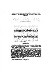
52 security requirements. It may take the form of delivery in person, by trusted courier or perhaps an electronic channel that they know is sufficiently secure during the transmission of the key. After the key has been exchanged, Alice then encrypts her message and the ciphertext is sent across insecure public channels where we assume there are eavesdroppers who may obtain the ciphertext. This information is reflected in Figure 4.1. If the parties are across town, a key may be delivered in person; however, should one wish to communicate with someone on another continent he has never met, the problem becomes much more difficult.

Eavesdropper

Message Transmission (Public Channel)

Alice

Key Transmission (Secure Channel)

Bob

Figure 4.1: Message And Key Transmission We refer to this as the key distribution problem and it was this obstacle which was a road block for the proliferation of secure communications. In their seminal paper [DH76], Whitfield Diffie and Martin Hellman revolutionized the science of cryptography by providing a method of exchanging keys over insecure public channels, completely obviating the need for a secure channel. Their idea was to use a one-way

53 function, which can informally be defined as a function f such that if we are given x in the domain of f , f (x) is easy to compute, but given y in the range of f , finding x such that f (x) = y is computationally difficult. In their paper, the one-way function they proposed for key exchange was exponentiation in a finite cyclic group. Reversing this operation is known as the Discrete Logarithm Problem (DLP). The problem is, given a finite cyclic group1 G generated by g, to quickly compute (deterministically in polynomial time) the integer x (with 0 ≤ x < |G| where |G| denotes the number of elements of G) given the element g x . A proof that this problem is a one-way function would require a proof that there does not exist a deterministic polynomial time algorithm that computes x. Since this problem can clearly be solved nondeterministically in polynomial time, a proof that a deterministic algorithm does not exist would also prove the well-known complexity theory conjecture that P = 6 N P.2 Because the DLP (nor any other problem) has not been proved to be a one-way function, the most we can say is that it has resisted the intensive efforts of many gifted mathematicians and only modest progress has been made toward a solution. Should Alice and Bob wish to exchange a key, the protocol is: 1. Agree on a finite cyclic group G and a generator g. (public) 2. Alice picks a random integer x with 0 < x < |G|. (secret) 3. Bob picks a random integer y with 0 < y < |G|. (secret) 4. Alice computes a = g x , and sends a to Bob. (public) 1

In fact, all that is required is a finite semi-group. P is the set of decision problems that can be solved deterministically in polynomial time and N P is the set of decision problems that can be solved nondeterministically in polynomial time. 2

54 5. Bob computes b = g y , and sends b to Alice. (public) 6. Alice computes k = bx . (secret) 7. Bob computes k 0 = ay . (secret) Since k = bx = (g y )x = g yx = g xy = (g x )y = ay = k 0 , they now share a common key. Note that an eavesdropper has all of the information required to compute the key, but since finding x given g x is computationally infeasible if |G| is large, the key may be considered secret.3 The focus of this thesis is on real quadratic fields but we mention that an imaginary quadratic field based key exchange was introduced by Buchmann and Williams in [BW88a]. This cryptosystem is based on a finite group, namely the class group. Here, Alice and Bob agree on a class group, which is specified by the imaginary √ quadratic field Q( D), and an element g of the group (an equivalence class). While each equivalence class contains an infinite number of elements, a unique reduced ideal exists in each class which may be considered the class representative. They exponentiate g as per the Diffie-Hellman protocol, and the key is based upon the reduced result. Imaginary quadratic field cryptography has been extensively studied by Buchmann and Hamdy in [BH01]. The majority of today’s popular cryptosystems rely on the difficulty of factoring or solving the DLP in a finite group. In [BW90], Buchmann and Williams introduced the first Diffie-Hellman type public-key exchange system not based on a finite group. 3

It should be mentioned that the Diffie-Hellman protocol might not actually require the DLP to be solved in order to break the system. If a fast method is found that can find g xy given g x and g y then the system is broken. This is referred to as the Diffie-Hellman problem and it is not known whether the Diffie-Hellman problem and DLP are equivalent. Certainly solving the DLP will break the Diffie-Hellman key exchange, but the converse might not be true.

55 Instead, it is based on the set of reduced principal ideals of a real quadratic field. We have closure on this set under the operation of multiplication followed by reduction; however, under this operation we lose associativity and hence we do not have a group. To pick a reduced representative from the set, we use Algorithm 3.5. Since this key exchange is not based on a group structure, it may possibly remain secure even if the DLP for finite groups is solved. The following is a theoretical key-exchange protocol utilizing ideals of the ring of integers of a real quadratic field. In practice, an exact representation of the relative generators cannot be sent because the size of the parameters defining them is exponential in D. Hence, an approximation such as the (f, p) representation of [JSW] must be used instead. This is explained further in Chapter 6. √ 1. Agree on a real quadratic field K = Q( D) where D > 0 is square-free and a reduced principal ideal g ∈ OK . (public) 2. Alice picks a random integer x with 0 < x
0, D is used. For a simple example, consider Qi = 28, Pi = 23, Ri = 17 and Di = bi = b28/22 c = 7, Pbi = b23/22 c = 5, R bi = b17/22 c = 4 and 53. If k = 2 then Q b i = 52 − (7)(4) = −3. Either the algorithm used in the single-precision reductions D b i must be used. Some must take this into account or a different computation for D possibilities are discussed in the following chapter. b i > 0 and Lagrange reduction (Algorithm 3.3) is used to reConceptually, if D bi , Pbi ), this procedure embeds the partial quotients [˜ duce (Q q0 , q˜1 , . . . , q˜j ] used in the

5.1. RICKERT’S ALGORITHM

60

bi , Pbi ) into the reduction of (Qi , Pi ) so that reduction of (Q √

√ # Pi + D Pi+1 + D = q˜0 , q˜1 , . . . , q˜j , . Qi Qi+1 "

bi , Pbi and R bi , if one of them is 0, or if When we compute the approximations Q bi , Pbi ) is a reduced ideal, a full multi-precision reduction step is taken on (Qi , Pi ) (Q instead, and then the procedure is continued with approximations. We continue this process until a fully reduced ideal ar is obtained. The procedure is given in detail as Algorithms 5.1 and 5.2.


Algorithm 5.1: Rickert–Style Reduction Algorithm (Matrix) Q0 P0 Input: A0 = ,D P0 R 0 Output: Ai , N such that Ai = φN (A0 ) and (Qi , Pi ) is reduced [ Initialization ] i←0 [ Reduction ] while (Qi , Pi ) is not reduced do k ← max(max(dlog 2 Qi e, dlog 2 Pi e, dlog2 Ri e) − (word size), 0) k k Q /2 P /2 b i ← i k i k A Pi /2 Ri /2 2 b b b b Di ← Pi − Qi Ri q b i is 0 or (Q bi , Pbi ) is reduced in Q b i then if an entry of A D [ Full$multi-precision reduction ] √ % Pi + D qi ← Qi qi −1 Ni ← −1 0 Ai+1 ← (−1)NiT Ai Ni else [ Single-precision reduction ] b i+1 , Ni ← Algorithm 3.2 or 3.6 (A b i, D b i) A Ai+1 ← (det Ni )NiT Ai Ni i←i+1 return Ai , N =

i−1 Y j=0

Nj

61


62

Algorithm 5.2: Rickert–Style Reduction Algorithm (Ideal) Input: a0 = (Q0 , P0 ), D Output: ai , Ψi such that ai = (Ψi )a0 and ai is reduced [ Initialization ] i←0 ψ0 ← 1 √ P02 − D R0 ← Q0 [ Reduction ] while ai is not reduced do k ← max(max(dlog i e, dlog2 Pi e, dlog2 Ri e) − (word size), 0) 2 Q k bi ← Ri /2k b b Qi ← Qi /2 , Pi ← Pi /2k , R bi R bi b i ← Pb2 − Q D i q bi , Pbi or R bi is 0 or (Q bi , Pbi ) is reduced in Q if one of Q

bi D

then

[ Full$multi-precision reduction ] √ % Pi + D qi ← Qi ψi+1 ← αi − qi else [ Single-precision reduction ] ψi+1 Relative generator (with α bi replaced by αi ) from reducing b ai in q← Q

bi D

using Algorithm 3.2 or 3.6.

ai+1 ← (ψi+1 )ai i←i+1 return ai , Ψi =

i Y j=0

ψj

¨ 5.2. SCHONHAGE’S ALGORITHM

5.2

63

Sch¨ onhage’s Algorithm

The divide and conquer technique was used by Schönhage [Sch91] to give an asymptotically fast method of reducing forms. We present the algorithm here in terms of ideals and show how to compute the relative generator. To use divide and conquer, the problem of reducing an ideal must be somehow split into smaller subproblems. The idea Schönhage had was to find an ideal that is minimal above some value s. Definition 5.1. (Q, P ) is minimal above above s > 0 if 1. Q, P, R ≥ s and 2. (a) Q − 2P + R < s or (b) P − Q < s and P − R < s . We will show that if an ideal is minimal above 1 then it is at most one step from being reduced. Before looking into the details of this method, we present an overview of the algorithm. To satisfy the first condition of Definition 5.1 for any value of s, we need Q, P and R positive to start with; this is accomplished with Algorithm 5.4. We then find an ideal minimal above 1. Lastly, we do the final reduction step and terminate. The main components are combined as Algorithm 5.3. The algorithm returns a reduced ideal and relative generator.

Make Q, P and R Positive The first step in making Q, P and R positive is to ensure Q + R > 0. If Q + R < 0 then negate Q, P and R. We obtain a rationale for this approach by considering the


64

Algorithm 5.3: Schönhage Reduction (Matrix) Q P Input: A = ,D P R Output: A0 , N such that A0 = φN (A) and (Q0 , P 0 ) is reduced

A0 , N1 sign ← Algorithm 5.4 (A) {Make positive} A0 , N2 , ← Algorithm 5.5 (A0 , −1) {Main reduction} A0 , N3 ← Algorithm 3.2 (A0 , D) {Final Lagrange reduction steps} N ← N 1 N2 N 3 A0 ← sign · A0 return A0 , N

associated matrix

Q P P R

. If

Q0 P 0 P 0 R0

= φN

Q P P R

then

−Q0 −P 0 −P 0 −R0

= φN

−Q −P −P −R

, that

is, the steps are the same to reduce (Q, P ) as to reduce (−Q, −P ). 0 1 Second, we want to ensure that P > 0. If P < 0, we use the matrix N = ( −1 0)

and corresponding function φN from Definition 3.4 to see that (Q, P ) ∼ (R, −P ). √ From Equation (3.4), this transformation is realized by (R, −P ) = D−P (Q, P ). Q At this point we know that Q + R > 0 which guarantees that at most one of Q or R is negative. If Q < 0, then using φN where N = ( 11 01 ) we set Q ← Q+2P +R, P ← P + R, and leave R unchanged. Since Q + R, P, and R were positive, we know the new values for Q, P, and R are positive. A similar argument works with the matrix N = ( 10 11 ) if R < 0. The full algorithm to make the ideal parameters positive is given as Algorithm 5.4.

Monotone Reduction To find an ideal minimal above 1 we use the divide and conquer MR algorithm (Algorithm 5.5). The first step is to partially reduce (Q, P ) until it is minimal above


65

Algorithm 5.4: Make Positive (Matrix) Q P Input: A = P R 0 Output: A , N , sign, such that all entries of A0 are positive and A0 = (sign)φN (A)

[ Initialization ] A0 ← A, N ← I2 [ Ensure Q0 + R0 ≥ 0 and P 0 ≥ 0 ] if (Q0 + R0 < 0) then A0 ← −A0 sign ← −1 else sign ← 1 if (P 0 0 ⇒ (P − Q) + (P − R) < 0 .

This implies that at most one of P − Q and P − R can be positive. Choosing the positive course, we have a unique reduction path. The Divide and Conquer technique requires a generalization of this idea. Instead of simply requiring that Q, P , and R be positive, we require that they be greater than 2m for some m ∈ Z. As we will soon show, this criterion also provides a unique reduction path and we observe from Definition 5.1 that once it is not possible to take a low step or high step without one of Q, P or R becoming less than 2m , (Q, P ) is minimal above 2m . Given Q, P, R > 2m ,

Q − 2P + R > 2m ⇒ (P − Q) + (P − R) < −2m ⇒ At most one of P − Q and P − R is greater than 2m .

Since a low step requires the calculation of P − Q and a high step requires P − R, only one of these steps satisfies the condition that all parameters be greater than 2m . We may make these steps more efficient by combining consecutive low steps as 1 −q 0 1 . This gives the formulas Q0 ← Q ,


70

P 0 ← P − qQ , R0 ← q 2 Q − 2qP + R .

We may find the optimal value of q so that all coefficients are greater than 2m by seeing that D = P 02 − QR0 ⇒ P 02 ≥ D + 2m Q, if R0 ≥ 2m . Now we have two conditions on P 0 :

p

0

1) P = P − qQ ≥ D + {z |

2m Q

P 02 ≥D+2m Q

2) P 0 =

P − qQ ≥ 2m | {z }

⇒ q≤

P−

√

} ⇒ q≤

D + 2m Q Q

P − 2m Q

minimal above constraint

Hence, the optimal value of q is

P −t q= , Q

p t = max( D + 2m Q, 2m ) .

Consecutive high steps may be combined with q found symmetrically as

P −t q= , R

√ t = max( D + 2m R, 2m ) .

Given Q, P and R, one combined set of low steps or one combined set of high steps is referred to as a simple step. Algorithms 5.6 and 5.7 perform the simple step operation. In the following chapter, the implementation is based on Algorithm 5.6 while Algorithm 5.7 is provided to clarify how the ideal and relative generator are affected by each simple step.


71

5.6: Simple Step Above 2m (Matrix) Algorithm Qi Pi Input: Ai = , m where (Qi , Pi ) is an ideal that is to be reduced one Pi R i simple step above 2m Output: Ai+1 , N such that Ai+1 = φN (Ai ) and (Qi+1 , Pi+1 ) has been reduced a simple step D ← Pi2 − Qi Ri {Store in a lookup table indexed by Qi , Pi , Ri } if (Pi > Qi ) then [ Low step√ ] m Q , 2m ) t ← max( D + 2 i Pi − t q← Qi 1 −q N← 0 1 else [ High step √] m R , 2m ) t ← max( D + 2 i Pi − t q← Ri 1 0 N← −q 1 Ai+1 ← N T Ai N return Ai+1 , N

Finishing The Reduction With these definitions in place, we are now able to show that if the MR algorithm is called with a value between 0 and 1 it yields an ideal within one step of being reduced. Proposition 5.2. An ideal (Q, P ) minimal above 1 is within one step of being reduced.


72

Algorithm 5.7: Simple Step Above 2m (Ideal) Input: ai = (Qi , Pi ), m Output: ai+1 = (Qi+1 , Pi+1 ), ψi+1 such that ai+1 = (ψi+1 )ai and ai+1 has been reduced a simple step above 2m D ← Pi2 − Qi Ri {Store in a lookup table indexed by Qi , Pi , Ri } if (Pi > Qi ) then [ Low step√ ] m Q , 2m ) t ← max( D + 2 i Pi − t q← Qi ψi+1 ← 1 else [ High step √] m R , 2m ) D + 2 t ← max( i Pi − t q← Ri ψi+1 ← 1 − q α ¯i ai+1 ← (ψi+1 )ai return ai+1 , ψi+1 Proof. Without loss of generality, assume Q < R.

D > 0 ⇒ P 2 > QR ⇒ P > Q

(D is not a square) .

Also, this implies that condition 2b of Definition 5.1 is impossible.

(Q, P ) minimal above 1 ⇒ Q − 2P + R < 1

(definition)

⇒ Q − 2P + R < 0

(D is not square)

⇒ R < 2P − Q

5.3. SCHNORR AND SEYSEN’S ALGORITHM ⇒ (P − Q)2 = P 2 − Q(2P − Q) < P 2 − QR = D √ ⇒ 0

Fast Ideal Arithmetic in Quadratic Fields - Semantic Scholar

Fast Ideal Arithmetic in Quadratic Fields - Semantic Scholar

Suggest Documents

Efficient Ideal Reduction in Quadratic Fields 1 Introduction - Google Sites

Efficient Ideal Reduction in Quadratic Fields 1 Introduction

The FAST Satellite Fields Instrument - Semantic Scholar

Arithmetic of Finite Fields

Fast Reduction of Ternary Quadratic Forms - Semantic Scholar

Graph-Based Quadratic Optimization: A Fast ... - Semantic Scholar

Quadratic programs with quadratic constraint ... - Semantic Scholar

Factoring in quadratic fields - UConn Math

SEVEN CONSECUTIVE PRIMES IN ARITHMETIC ... - Semantic Scholar

Incomplete Reduction in Modular Arithmetic - Semantic Scholar

SEVEN CONSECUTIVE PRIMES IN ARITHMETIC ... - Semantic Scholar

Leak Resistant Arithmetic - Semantic Scholar

NOTES ON PRIMES IN ARITHMETIC ... - Semantic Scholar

SEVEN CONSECUTIVE PRIMES IN ARITHMETIC ... - Semantic Scholar

External Representations in Arithmetic Problem ... - Semantic Scholar

Monetary Policy Arithmetic - Semantic Scholar

Lambda-Lifting in Quadratic Time - Semantic Scholar

Application of The Quadratic Almost Ideal Demand

Fast Arithmetic in Algorithmic Self-Assembly

BLOCK STRUCTURED QUADRATIC ... - Semantic Scholar

Ideal Convergence in Generalized Topological ... - Semantic Scholar

Ideal Cooperation in Dialogues - Semantic Scholar

Gaussian fields - Semantic Scholar

on certain problems in the analytical arithmetic of quadratic forms