faster than an Expectation-Maximization method for Gamma mixture models, our ... provide a new algorithm for Gamma mixtures which is faster than methods.
Fast learning of Gamma mixture models with k-MLE Olivier Schwander1 and Frank Nielsen2 1
2
École Polytechnique, Palaiseau, France Sony Computer Science Laboratories, Tokyo, Japan
Abstract. We introduce a novel algorithm to learn mixtures of Gamma distributions. This is an extension of the k-Maximum Likelihood estimator algorithm for mixtures of exponential families. Although Gamma distributions are exponential families, we cannot rely directly on the exponential families tools due to the lack of closed-form formula and the cost of numerical approximation: our method uses Gamma distributions with a fixed rate parameter and a special step to choose this parameter is added in the algorithm. Since it converges locally and is computationally faster than an Expectation-Maximization method for Gamma mixture models, our method can be used beneficially as a drop-in replacement in any application using this kind of statistical models.
1
Introduction and prior work
Statistical mixtures are among the most used tools in many applications which require to model experimental data with probability distributions. Such a mixture is a weighted sum of components which are themselves probability distributions (usually the same distribution is shared by all the components):
m(x) =
k X
ωi p(x; θi )
(1)
i=1
The big challenge here is to learn the parameter vectors ω and θ and the number of components k (we limit us to the case of finite mixtures but some algorithms may output mixtures with an infinite number of components [1]). One of the most famous algorithms to learn the parameters ω and θ is the ExpectationMaximization (EM) algorithm [2]. We address here the problem of learning mixtures of Gamma distributions (see Fig. 1)). Although not as common as Gaussian mixture models, Gamma mixtures are of interest in many applications as various as bioinformatics [3], communication networks modeling [4] or health services analysis [5] and a lot of work has been devoted to these mixtures. Our new algorithm is an extension of the k-Maximum Likelihood estimator (k-MLE) algorithm by Nielsen [6]. It relies on the same principle which was already used for mixtures of generalized Gaussians [7]. Our contribution is to
0.12 0.10 0.08 0.06 0.04 0.02 0.000
5
10
15
20
25
Fig. 1. A mixture of Gamma distributions with 3 components: ω1 = 0.12, α1 = 1, β1 = 1; ω2 = 0.4, α2 = 4, β2 = 2; ω3 = 0.48, α3 = 30, β3 = 0.5.
provide a new algorithm for Gamma mixtures which is faster than methods based on Expectation-Maximization Since the studied method relies on the exponential families framework, the necessary background about exponential families is recalled and we show that Gamma distributions are members of the exponential families. After a description of two algorithms designed to learn mixtures of exponential families, Bregman Soft Clustering, which relies on EM and k-MLE, we explain why they are not well suited for the particular case of Gamma mixtures. In the following section we present our extension of k-MLE which allows to efficiently learn mixtures of Gamma distributions. In the last section we evaluate the effectiveness of our proposed algorithm both in terms of computational cost and in terms of quality of the produced models.
2 2.1
Exponential families and their parametrizations Definition
Exponential families are a widespread class of distributions and many commonly used distributions belong to this class (with the notable exception of the uniform distribution): for example Gaussian, Beta, Gamma, Rayleigh, Von Mises are all members of this class ([8] provides a vast list of exponential families with their decomposition). An exponential family is a set of probability mass or probability density functions which admits the following canonical decomposition: p(x; θ) = exp(ht(x), θi − F (θ) + k(x)) with – t(x) the sufficient statistic, – θ the natural parameters, – h·, ·i the inner product,
(2)
– F the log-normalizer, – k(x) the carrier measure. The log-normalizer characterizes the exponential family and is equal to: Z F (θ) = log
exp(ht(x), θi + k(x)) dx
(3)
x
Since this log-normalizer F is a strictly convex and differentiable function, it admits a dual representation by the Legendre-Fenchel transform: F ? (η) = sup {hθ, ηi − F (θ)}
(4)
θ −1
We get the maximum for θ = (∇F )
(η) and F ? can be computed with:
F ? (η) = hη, θi − F (θ)
(5)
Thus we deduce that the gradient of F and of its dual F ? are inversely reciprocal: ∇F = (∇F ? )
−1
(6)
The duality between F and its Legendre transform F ? leads to a new parametrization for the exponential families, which is the dual of the natural parameters: the so-called expectation parameters η = ∇F (θ). The parameters η are called expectation parameters since η = E [t(x)] [8]. In the general case, the dual F ? may be not known in closed-form and thus may require numerical approximation (which is time consuming and submitted to various practical problems like the choice of the initialization for an iterative procedure). 2.2
Bregman divergences
Bregman divergences are a family of divergences parametrized by the set of strictly convex and differentiable functions and is written as: BF (pkq) = F (p) − F (q) − hp − q, ∇F (q)i
(7)
The function F is called the generator of the Bregman divergence. The family of Bregman divergences generalizes a lot of usual divergences, for example: – the squared Euclidean distance, for F (x) = x2 , – the Kullback-Leibler (KL) divergence, with the Shannon negative entropy Pd F (x) = i=1 xi log xi (also called Shannon information).
2.3
Bijection between exponential families and Bregman divergences
Banerjee et al. [9] showed that Bregman divergences are in bijection with the exponential families through the generator F . For each exponential family with a log-normalizer F there is one and only one Bregman divergence whose generator is F ? , the Legendre dual of F . We can rewrite the exponential family in terms of the corresponding Bregman divergence:
p(x; θ) = exp(ht(x), θi − F (θ) + k(x)) = exp(−B
F?
(8)
?
(t(x)kη) + F (t(x)) + k(x))
(9)
where η is the expectation parameter of the family (η = ∇F (θ)). This bijection allows in particular to compute the Kullback-Leibler divergence between two members of the same exponential family: Z KL (p(x, θ1 ); p(x, θ2 )) =
p(x; θ1 ) log x
p(x; θ1 ) dx p(x; θ2 )
=BF (θ2 kθ1 )
(10) (11)
where F is the log-normalizer of the exponential family and the generator of the associated Bregman divergence. Thus, computing the Kullback-Leibler divergence between two members of the same exponential family is equivalent to computing a Bregman divergence between their natural parameters (with swapped order). 2.4
Gamma is an exponential family
The general case of the Gamma distribution is
p(x; α, β) =
β α xα−1 exp(−βx) Γ (α)
(12)
with α, β > 0 and x is a positive real number. The parameter α is called the shape parameter and β is called the rate parameter (or inverse scale parameter). It is common to find another parametrization which replace the rate parameter by the scale parameter θ = β1 . This distribution is an exponential family with the following parametrization: Natural parameters (θ1 , θ2 ) = (−β, α − 1) Sufficient statistics t(x) = (x, log x)
Log normalizer F (θ1 , θ2 ) = (−(θ2 + 1) log(−θ1 ) + log Γ (θ2 + 1))
Gradient log normalizer ∇F (θ1 , θ2 ) =
�
θ2 +1 −θ1 , − log(−θ1 )
+ ψ(θ2 + 1)
�
� � Dual log normalizer F ? (η1 , η2 ) = (∇F )−1 (η1 , η2 ), (η1 , η2 ) −F (∇F )−1 (η1 , η2 )
Although the log-normalizer F and its gradient ∇F are known in closed-form, −1 it is not the case for its dual F ? and for the gradient of the dual ∇F ? = (∇F ) . It thus requires numerical approximation, which is computationally costly.
3 3.1
Learning mixtures of exponential families Bregman Soft Clustering
The Bregman Soft Clustering for mixtures of exponential families has been introduced in [9]. It is actually a meta-algorithm which takes the considered family as an input of the algorithm and which does not require specific adaptation for each family, contrary to most of the previously proposed methods. As a variant of EM, it still relies on the usual two steps: Expectation step: The usual Expectation-Maximization algorithm gives us the following formulation for the posterior probabilities: ωi p(xt ; ηi ) p(i|xt , η) = Pk j=1 ωj p(xt ; ηj )
(13)
Using the bijection between exponential families, we can replace the probability density function of the exponential family by its expression using the associated Bregman divergence. ωi exp (−BF ? (t(xi )kηi )) exp k(xt ) p(i|xt , η) = Pk ? j=1 ωj exp (−BF (t(xt )kηj )) exp k(xt )
(14)
ωi exp (−BF ? (t(xt )kηi )) = Pk ? j=1 ωj exp (−BF (t(xt )kηj ))
(15) (16)
Since BF ? (pkq) = F ? (p) − F ? (q) − hp − q, ∇F ? (q)i we can expand the expression of the Bregman divergence in the previous expression:
p(i|xt , η) = Pk
ωi exp (−F ? (t(xt )) − F ? (ηi ) − ht(xt ) − ηi , ∇F ? (ηi )i)
j=1
= Pk
ωj exp (−F ? (t(xt )) − F ? (ηj ) − ht(xt ) − ηj , ∇F ? (ηj )i)
ωi exp (F ? (ηi ) + ht(xt ) − ηi , ∇F ? (ηi )i)
j=1
ωj exp (F ? (ηj ) + ht(xt ) − ηj , ∇F ? (ηj )i)
(17) (18)
Maximization step: The maximization step is done with the maximum likelihood estimator for exponential families [9]. It can be computed as the average of the sufficient statistics on the observations:
ηˆ = E [t(x)] =
1X t(xi ) n
(19)
Notice that we get an estimate which lives in the space of the expectation parameters. If one wants the associated natural parameter θˆ = ∇F ? (ˆ η ), the ∇F ? function will be needed, either in closed-form or with a numerical approximation (which will be computationally costly). 3.2
k-Maximum Likelihood Estimator
Assume we have a set X = {x1 , . . . , xn } of n observations which have been sampled from a finite mixture model with k components. The joint probability distribution of theses samples with the missing components zi (indicating from which component each observation xi comes from) is: p(x1 , z1 , . . . , xn , zn ) =
Y
p(zi |ω)p(xi |zi , θ)
(20)
i
Since the variables zi are not observed in practice, we marginalize these variable and we get: p(x1 , . . . , xn |ω, θ) =
YX i
p(zi = j|ω)p(xi |zi = j, θ)
(21)
j
The straightforward way to optimize this distribution would be to test the k n labels but this is not tractable in practice. Instead, Expectation-Maximization optimizes the following quantity, the expected log-likelihood: ¯l(x1 , . . . , xn ) = 1 log p(x1 , . . . , xn ) n X 1X log p(zi = j|ω)p(xi |zi = j, θ) = n i j
(22) (23)
Contrary to this approach, the k-Maximum Likelihood Estimator maximizes the average complete log-likelihood: ¯l0 (x1 , z1 , . . . , xn , zn ) = 1 log p(x1 , z1 , . . . , xn , zn ) n � Y� 1X δ(z ) log (ωj pF (xi , θj )) i = n i j =
1 XX δ(zi ) (log pF (xi , θj ) + log ωj ) n i j
(24) (25) (26)
Since pF is an exponential family, we have: log pF (xi , θj ) = −BF ∗ (t(x), ηj ) + F ? (t(x)) + k(x) | {z }
(27)
does not depend on θ
The terms which do not depend on θ are of no interest for the maximization problem and can be removed: we can then rewrite Eq. (26) to get the equivalent problem: arg min
XX i
δ(zi ) (BF ∗ (t(x), ηj ) − log ωj )
(28)
j
As stated in [6] this problem can be solved for a fixed set of weights ωi using the Bregman k-means algorithm with the Bregman divergence BF ∗ (actually, any heuristic for k-means is convenient). The weights can now be optimized by taking ωi = |Cni | (where |Ci | is the number of observations put in the cluster Ci by the solution of the previous clustering problem). This step amounts to maximize the cross-entropy of the mixture [6]. The full algorithm can be summarized as follows (see Fig. 2(a) for a block diagram): 1. Initialization (random or using k-MLE ++[6]); 2. Assignment zi = arg maxj log(ωj pF (x Pi |θj )); 3. Update of the η parameters ηi = n1j x∈Cj t(xi ); Goto step 2 until local convergence; 4. Update of the parameters ω j ; Goto step 2 until local convergence of the complete likelihood.
4 4.1
k-MLE for Gamma Gamma with fixed rate parameter
The algorithms described in the two previous sections needs frequent conversions between natural parameters θ and expectation parameters η. The bijection between the two parameter spaces uses the functions ∇F and ∇F ? which are not
Assignment
Update parameters
Update weights
Until convergence
Until convergence
Assignment
Update parameters
Until convergence
Initialization
Until convergence
Initialization
Choose family Update weights
(a) Original k-MLE
(b) Extended k-MLE
Fig. 2. Block diagram for the original algorithm and its extension
known in closed-form for the Gamma distribution. Moreover, the evaluation of the Bregman divergence BF ? is also needed, but the function F ? is also missing in closed-form. k-MLE may still be applicable to Gamma mixtures but the numerical approximations needed would dramatically reduce the speed of the algorithm, which is one of its main interests [10]. To avoid the computational difficulties for the functions which are not known in closed form, we introduce the Gamma distribution with a fixed rate parameter. The parameter β is not any more a member of the source parametrization and is instead a parameter of the distribution.
pβ (x; α) =
β α xα−1 exp(−βx) Γ (α)
(29)
This is still an exponential family with the following parametrization (a comprehensive list of formulas is given in Table 1): Natural parameters θ = α − 1 Log normalizer F (θ) = −(θ + 1) log(β) + log Γ (θ + 1)
Gradient log normalizer ∇F (θ) = − log(β) + ψ(θ + 1) Dual log normalizer F ? (η) = h∇F ? (η), ηi − F (∇F ? (η)) Gradient of the dual log normalizer ∇F ? (η) = (∇F )−1 (η)
The ∇F function can be inverted in closed-form with respect to the inverse digamma function ψ −1 , giving: (∇F )−1 (η) = ψ −1 (η + log β) − 1 = ∇F ? (η)
(30)
We can now compute the F ? function by directly applying the Legendre transform to the log-normalizer F : F ? (η) = h∇F ? (η), ηi − F (∇F ? (η)) −1
(η + log β) − 1) + ψ � − log Γ ψ −1 (η + log β)
= η (ψ
(31) −1
(η + log β) log β
(32)
Strictly speaking, this is still not a closed-form but, contrary to the functions we get for the full Gamma distribution, the two missing functions Γ and ψ −1 can be computed efficiently: algorithms for the Γ function are well known [11] and ψ −1 is numerically well behaved and can be computed efficiently computed with a dichotomic search 3 . 4.2
Maximum likelihood estimator
Results from exponential families [9] give an estimator for the expectation parameters of the fixed rate family:
ηˆ =
1X 1X t(xi ) = log(xi ) = − log α ˆ + ψ(β) n n
(33)
By derivation of the likelihood function, we get an estimator for the rate parameter β [4]: nˆ α βˆ = P xi 3
(34)
See http://hips.seas.harvard.edu/files/invpsi.m for a working Matlab implementation which can be easily translated in any language
β α xα−1 exp(−βx) Γ (α)
PDF
pβ (x; α) =
Λ→Θ
θ =α−1
Θ→Λ
α=θ+1
Λ→H
η = − log β + ψ(α)
H→Λ
α = ψ −1 (η + log β)
Θ→H
η = ∇F (θ)
H→Θ
θ = ∇F ? (η)
Log normalizer
F (θ) = −(θ + 1) log β + log Γ (θ + 1)
Gradient log normalizer
∇F (θ) = − log β + ψ(θ + 1)
Dual log normalizer
F ? (η) = η(ψ −1 (η + log β) − 1) + ψ −1 (η + log β) log β + log Γ (ψ −1 (η + log β))
Gradient dual log normalizer ∇F ? (η) = ψ −1 (η + log β) − 1 Sufficient statistic
t(x) = log x
Carrier measure k(x) = −βx Table 1. Gamma distribution with fixed rate as an exponential family
4.3
Learning mixtures
The original k-MLE algorithm builds mixture models where all the components belong to the same exponential family. Although generic Gamma distributions are exponential families, Gamma distributions with fixed rate are not in the same exponential family if the rate parameter is not the same across components. In order to build a mixture with a different β parameter for each component, we will follow the approach introduced in [7] (for generalized Gaussian) which adds a supplementary step to the k-MLE procedure (see Fig. 2(b)): before updating the weights, the family of each component is chosen using a maximum likelihood estimator. In the Gamma case, it amounts to choosing the rate parameter of each component, using the MLE given in Eq. (34). The new k-MLE algorithm for Gamma mixtures (k-MLE-Gamma) can be summarized as follows: 1. Initialization (random or using k-MLE ++[6]); 2. Assignment zi = arg maxj log(ωj pFj (xi |θj )); P 3. Update of the η parameters ηi = n1j x∈Cj log(xi ); Goto step 2 until stability (local convergence of the k-means); 4. Update of the parameters ω j and β j (for all j); Goto step 2 until local convergence of the complete likelihood.
4.4
Convergence to a local maximum
As the one proposed for generalized Gaussian, this algorithm converges to a local maximum of the complete log-likelihood. We want to minimize the same cost function as the original k-MLE algorithm, the complete log-likelihood of the mixture, with the slight difference that the log-normalizer is not shared among components but now depends on the values βj and is now written Fj instead of F:
¯l(x1 , z1 , ..., xn , zn |w, θ) = 1 n =
n X k X
δj (zi )(log pFj (xi |θj ) + log ωj )
(35)
i=1 j=1
n k � 1 XX δj (zi ) − BFj ∗ (t(xi ), ηj ) n i=1 j=1 � + Fj ∗ (t(xi )) + kj (xi ) + log ωj
(36)
Let Cj be the set of the indices of the observations sampled from the j-th component. Maximizing the log-likelihood ¯l is equivalent to minimizing the cost function −¯l: k
XX ¯l0 = −¯l = 1 Uj (xi , ηj ) n j=1
(37)
i∈Cj
where
Uj (xi , ηj ) = − log pFj (xi |θj ) + log ωj ∗
�
= BFj ∗ (t(xi ) : ηj ) − Fj (t(xi ))
(38) (39)
− kj (xi ) − log ωj is the cost for the observation i to have been sampled from the component j. Notice this cost depends on j since each component has a different generator Fj and a different carrier measure kj . This minimization problem can be solved with the Lloyd k-means algorithm [12] using the cost function U (which is not a distance nor a divergence and can even be negative). A proof of the convergence of the Lloyd algorithm for this cost function is given in [7]. After the execution of the Lloyd algorithm, the log-likelihood has been optimized for fixed ωj and βj . The final step is to update these two parameters using the proportion of samples in each cluster for the weights and the estimator for β (from Eq. (34)).
5
Expectation-Maximization for Gamma mixtures
Almhana et al. [4] proposed a specific variant of Expectation-Maximization for Gamma mixtures. The E step is unchanged compared to the classical EM algorithm, the only changes are in the M step: a specific update step is used for the α and β parameters. We will use this algorithm as a reference in the experiments presented in Section 6. Maximization step Given the current estimate for the parameters ω, α and β, the new values can be computed with: n
(k+1)
ωi
(k+1)
βi
(k+1)
αi
1X p(i|xt , θ(k) ) n t=1 (k) Pn (k) αi ) t=1 p(i|xt , θ = P n (k) ) t=1 xt p(i|xt , θ 1 (k) = αi + G k =
(40)
(41) (42)
with n
G=
6 6.1
� 1 X� (k) (k) log xt + log βi − ψ(αi ) p(i|xt , θ(k) ) n t=1
(43)
Experiments On synthetic data
The first experiment evaluates the convergence of k-MLE and the convergence of EM on a synthetic example: 15000 observations are sampled from a known three components Gamma mixture and the two evaluated methods are used to estimate Gamma mixture models with three components. We draw in Fig. 3 the log-likelihood of each mixture at each iteration of the two algorithms. Although the goal of k-MLE is to maximize the complete log-likelihood (Eq. (24)) and not the log-likelihood (Eq. (22) we see that both algorithms converge to a (local) maximum of the log-likelihood. Moreover k-MLE provides better results and converges way faster than EM. 6.2
On a real dataset
The second experiment describes experimental results on a real dataset which collects distances between atoms inside RNA molecules in order to predict the 3D structure of these molecules. Gaussian mixture models were successfully used to model the density of these distance [13] [14] but since the observations are
3.02 3.04 3.06 3.08 3.10 3.12 3.14 3.16 3.180
20
40
60
80
100
Fig. 3. Log-likelihood with respect to the number of components for k-MLE (dashed curve) and EM (plain curve). Higher curve (k-MLE model) means better model.
1.4
1.02
1.2
1.00
1.0
0.98
0.8
0.96
0.6
0.94
0.4
0.92
0.2
0.904
0.04
8
12
16
(a) Log-likelihood ratio
8
12
16
(b) Time ratio
Fig. 4. Log-likelihood and computation time ratios for k-MLE (right red bars) and EM (left blue bars) with respect to the number of components in the mixture. EM is our reference for comparison and thus has the score 1.
intrinsically positive a mixture model with a positive support (remember that Gaussian distribution is defined on R whereas the Gamma distribution is defined on R+ ) would be more statistically meaningful. Fig. 4 presents results on this dataset, in terms of log-likelihood and computation time with respect to the number of components in the mixture (4, 8, 12 and 16 components). Since absolute value for likelihood and time are difficult to compare meaningfully, we plot the mean ratio between the values got with k-MLE and the one got with EM (which is our reference for comparison and represented by 1 on the graphics). We see that k-MLE for Gamma mixtures performs similarly (or even better) to EM for Gamma mixtures for the quality of the built models and outperforms EM for the computation time (between 10% and 40%). The only case where k-MLE is worse than EM is for 4 components: k-MLE seems to be less robust when the number of components is not enough to model accurately the observations.
7
Conclusion
We presented a new algorithm for mixtures of Gamma distributions which is both fast and accurate. Accuracy is important since it means that the quality of the produced models (and thus the performances in the considered applications) will not decrease: our new algorithm could thus be considered as a drop-in replacement for other Gamma mixtures algorithms. The faster speed not only means that the computation time will decrease in applications where Gamma mixtures are already used but also that these mixtures will become of new interest in areas where the use of the Gamma distribution was theoretically interesting but not feasible in practice due to the high computation time. Moreover, this new extension of the k-Maximum Likelihood estimator shows the power and the genericity of the method which allows interesting perspectives for new and unexplored kinds of mixtures. Acknowledgments Thanks to the anonymous referees for their insightful comments and their careful proofreading.
References 1. Neal, R.M.: Markov chain sampling methods for dirichlet process mixture models. Journal of Computational and Graphical Statistics 9(2) (2000) 249–265 2. Dempster, A.P., Laird, N.M., Rubin, D.B.: Maximum likelihood from incomplete data via the EM algorithm. Journal of the Royal Statistical Society. Series B (Methodological) (1977) 1–38 3. Mayrose, I., Friedman, N., Pupko, T.: A Gamma mixture model better accounts for among site rate heterogeneity. Bioinformatics 21(Suppl 2) (2005) 4. Almhana, J., Liu, Z., Choulakian, V., McGorman, R.: A recursive algorithm for gamma mixture models. In: IEEE International Conference on Communications, 2006. ICC ’06. Volume 1. (June 2006) 197–202
5. Venturini, S., Dominici, F., Parmigiani, G.: Gamma shape mixtures for heavytailed distributions. The Annals of Applied Statistics 2(2) (June 2008) 756–776 Zentralblatt MATH identifier: 05591297; Mathematical Reviews number (MathSciNet): MR2524355. 6. Nielsen, F.: k-MLE: A fast algorithm for learning statistical mixture models. CoRR (2012) 7. Schwander, O., Schutz, A.J., Nielsen, F., Berthoumieu, Y.: k-MLE for mixtures of generalized Gaussians. In: 2012 21st International Conference on Pattern Recognition (ICPR). (November 2012) 2825–2828 8. Nielsen, F., Garcia, V.: Statistical exponential families: A digest with flash cards. CoRR 09114863 (2009) 9. Banerjee, A., Merugu, S., Dhillon, I.S., Ghosh, J.: Clustering with Bregman divergences. The Journal of Machine Learning Research 6 (2005) 1705–1749 10. Nielsen, F.: K-MLE: A fast algorithm for learning statistical mixture models. In: 2012 IEEE International Conference on Acoustics, Speech and Signal Processing (ICASSP). (March 2012) 869–872 11. Press, W.H., Teukolsky, S.A., Vetterling, W.T., Flannery, B.P.: Numerical recipes 3rd edition: The art of scientific computing. Cambridge University Press (2007) 12. Lloyd, S.P.: Least squares quantization in PCM. IEEE Transactions on Information Theory 28(2) (1982) 129–137 13. Sim, A.Y., Schwander, O., Levitt, M., Bernauer, J.: Evaluating mixture models for building rna knowledge-based potentials. Journal of Bioinformatics and Computational Biology 10(02) (2012) 14. Bernauer, J., Huang, X., Sim, A.Y., Levitt, M.: Fully differentiable coarse-grained and all-atom knowledge-based potentials for rna structure evaluation. RNA 17(6) (2011) 1066–1075