Fast Marching farthest point sampling for point clouds and implicit ...

Technical Report

UCAM-CL-TR-565 ISSN 1476-2986

Number 565

Computer Laboratory

Fast Marching farthest point sampling for point clouds and implicit surfaces Carsten Moenning, Neil A. Dodgson

May 2003

15 JJ Thomson Avenue Cambridge CB3 0FD United Kingdom phone +44 1223 763500 http://www.cl.cam.ac.uk/

c 2003 Carsten Moenning, Neil A. Dodgson

Technical reports published by the University of Cambridge Computer Laboratory are freely available via the Internet: http://www.cl.cam.ac.uk/TechReports/ Series editor: Markus Kuhn ISSN 1476-2986

Fast Marching farthest point sampling for point clouds and implicit surfaces Carsten Moenning and Neil A. Dodgson Abstract In a recent paper [13], the Fast Marching farthest point sampling strategy (FastFPS) for planar domains and curved manifolds was introduced. The version of FastFPS for curved manifolds discussed in the paper [13] deals with surface domains in triangulated form only. Due to a restriction of the underlying Fast Marching method, the algorithm further requires the splitting of any obtuse into acute triangles to ensure the consistency of the Fast Marching approximation. In this paper, we overcome these restrictions by using M´emoli and Sapiro’s [11, 12] extension of the Fast Marching method to the handling of implicit surfaces and point clouds. We find that the extended FastFPS algorithm can be applied to surfaces in implicit or point cloud form without the loss of the original algorithm’s computational optimality and without the need for any preprocessing.

1

Introduction

In Moenning and Dodgson [13], the notion of Fast Marching farthest point sampling (FastFPS) for planar domains and triangulated curved manifolds is put forward. FastFPS makes use of Fast Marching [23, 24] for the incremental construction of uniform or nonuniform distance maps across the sampling domain. As a result, an efficient progressive sampling method based on the uniform farthest point principle introduced by Eldar et al. [5, 6] and sharing its favourable properties such as excellent anti-aliasing properties, a high data acquisition rate and an elegant relationship to the Voronoi diagram concept is obtained. In addition, FastFPS provides a natural extension of the farthest point principle to the case of non-uniform, adaptive progressive sampling without the loss of computational optimality. A sampling technique featuring these properties is of particular interest for applications such as progressive transmission of image or 3D surface data [10], (progressive) rendering [14, 26], progressive acquisition [13] and machine vision [27]. FastFPS for triangulated surfaces requires the splitting of any obtuse into acute triangles in a preprocessing step [13]. Although this preprocessing step does not add significantly to the algorithm’s computational complexity, it affects its accuracy [7]. Furthermore, numerical analysis over polygonal surfaces is generally less accurate and robust than numerical analysis over Cartesian grids [4]. Finally, the surface domain may not be readily available in triangulated form or the computation of a triangulation may involve a performance penalty since it may otherwise not be required by the application. Using M´emoli and Sapiro’s [11, 12] recent augmentation of the Fast Marching concept, we propose an extended FastFPS method which may be applied to surfaces in implicit or 3

point cloud form without the need for any preprocessing or prior triangulation. Surfaces given in triangulated form may be dealt with by either using FastFPS for triangulated surfaces [13] or implicitising the surface in a preprocessing step. The method works on a Cartesian grid and retains the efficiency of FastFPS for triangulated surfaces [13]. We briefly review both the Voronoi diagram and the farthest point sampling as well as the “conventional” Fast Marching concept and its extension suggested by M´emoli and Sapiro [11, 12]. We then introduce our FastFPS algorithm for implicit surfaces and point clouds and present a worked example for its application to point clouds. We conclude with a brief summary and discussion.

2 2.1

Previous Work Voronoi diagrams

Given a finite number n of distinct data sites P := {p1 , p2 , . . . , pn } in the plane, for pi , pj ∈ P , pi 6= pj , let B(pi , pj ) = {t ∈ R2 |d(pi − t) = d(pj − t)}

(1)

where d may be an arbitrary distance metric provided the bisectors with regard to d remain curves bisecting the plane. B(pi , pj ) is the perpendicular bisector of the line segment pi pj . Let h(pi , pj ) represent the half-plane containing pi bounded by B(pi , pj ). The Voronoi cell of pi with respect to point set P , V (pi , P ), is given by \ V (pi , P ) = h(pi , pj ) (2) pj ∈P,pj 6=pi

That is, the Voronoi cell of pi with respect to P is given by the intersection of the halfplanes of pi with respect to pj , pj ∈ P , pj 6= pi . If pi represents an element on the convex hull of P , V (pi , P ) is unbounded. For a finite domain, the bounded Voronoi cell, BV (pi , P ), is defined as the conjunction of the cell V (pi , P ) with the domain. The boundary shared by a pair of Voronoi cells is called a Voronoi edge. Voronoi edges meet at Voronoi vertices. The Voronoi diagram of P is given by VD(P ) =

[

V (pi , P )

(3)

pi ∈P

The bounded Voronoi diagram, BVD(P ), follows correspondingly as: [ BVD(P ) = BV (pi , P )

(4)

pi ∈P

Figure 1 shows an example of a bounded Voronoi diagram. Note that the Voronoi diagram concept extends to higher dimensions. For more detail, see the comprehensive treatment by Okabe et al. [15] or the survey article by Aurenhammer [2]. 4

Figure 1: Bounded Voronoi diagram of 12 sites in the plane.

2.2

Farthest point sampling

Farthest point sampling is based on the idea of repeatedly placing the next sample point in the middle of the least-known area of the sampling domain. In the following, we summarise the reasoning underlying this approach for both the uniform and non-uniform case presented in Eldar et al. [5, 6]. Starting with the uniform case, Eldar et al. [5, 6] consider the case of an image representing a continuous stochastic process featuring constant first and second order central moments with the third central moment, i.e., the covariance, decreasing (exponentially) with spatial distance. That is, given a pair of sample points pi = (xi , yi ) and pj = (xj , yj ), the points’ correlation, E(pi , pj ), is assumed to decrease with the Euclidean distance, dij , between the points E(pi , pj ) = σ 2 e−λdij (5) p with dij = (xi − xj )2 + (yi − yj )2 . Based on their linear estimator, the authors subsequently put forward the following representation for the mean square error, i.e., the deviation from the “ideal” image resulting from estimation error, after the N th sample ZZ 2 ε (p0 , . . . , pN −1 ) = σ 2 − U T R−1 U dx dy (6) where Rij = σ 2 e−λ

√

and 2 −λ

Ui = σ e

(xi −xj )2 +(yi −yj )2

√

(xi −x)2 +(yi −y)2

5

for all 0 ≤ i, j ≤ N − 1. The assumption of stationary first and second order central moments has therefore yielded the result that the expected mean square (reconstruction) error depends on the location of the N + 1th sample only. Since stationarity implies that the image’s statistical properties are spatially invariant and given that point correlations decrease with distance, uniformly choosing the N + 1th sample point to be that point which is farthest away from the current set of sample points therefore represents the optimal sampling approach within this framework. This sampling approach is intimately linked with the incremental construction of a Voronoi diagram over the image domain. To see this, note that the point farthest away from the current set of sample sites, S, is represented by the centre of the largest circle empty of any site si ∈ S. Shamos and Hoey [25] show that the centre of such a circle is given by a vertex of the bounded Voronoi diagram of S, BVD(S ). Thus, as indicated in figure 2, incremental (bounded) Voronoi diagram construction provides sample points progressively.

Figure 2: The next farthest point sample (here: sample point 13) is located at the centre of the largest circle empty of any other sample site. From visual inspection of images it is clear that usually not only the sample covariances but also the sample means and variances vary spatially across an image. When allowing for this more general variability and thus turning to the design of a non-uniform, adaptive sampling strategy, the assumption of sample point covariances decreasing, exponentially or otherwise, with point distance remains valid. However, since Voronoi diagrams in non-uniform metrics may lose favourable properties such as cell connectedness, Eldar et al. [5, 6] opt for the non-optimal choice of augmenting their model by an applicationdependent weighting scheme for the vertices in the Euclidean Voronoi diagram. 6

2.3

Fast Marching

Fast Marching represents a very efficient technique for the solution of front propagation problems which can be formulated as boundary value partial differential equations. We show that the problem of computing the distance map across a smooth sampling domain can be posed in the form of such a partial differential equation and outline the Fast Marching approach towards approximating its solution. For simplicity, take the case of an interface propagating with speed function F (x, y, z) away from a source (boundary) point (u, v, w) across a 3D Euclidean domain. When interested in the time of arrival, T (x, y, z), of the interface at grid point (x, y, z), i.e., the distance map T given source point (u, v, w), the relationship between the magnitude of the distance map’s gradient and the given weight F (x, y, z) at each point can be expressed as the following boundary value formulation |∇T (x, y, z)| = F (x, y, z)

(7)

with boundary condition T (u, v, w) = 0. That is, the distance map gradient is proportional to the weight function. The problem of determining a weighted distance map has therefore been transformed into the problem of solving a particular type of Hamilton-Jacobi partial differential equation, the Eikonal equation [8]. For F (x, y, z) > 0, this type of equation can be solved for T (x, y, z) using Fast Marching. Since the Eikonal equation is well-known to become non-differentiable through the development of corners and cusps during propagation, the Fast Marching method considers only upwind, entropy-satisfying finite difference approximations to the equation thereby consistently producing weak solutions. As an example for a first order appromixation to the gradient operator, consider [18]  −x +x max(Dijk T, −Dijk T, 0)2 + −y +y max(Dijk T, −Dijk T, 0)2 + 1/2 −z +z max(Dijk T, −Dijk = Fijk T, 0)2 T

−T

(8) T

−T

+x −x T ≡ i+1jkh ijk are the where Fijk ≡ F (i∆x, j∆y, k∆z). Dijk T ≡ ijk h i−1jk and Dijk standard backward and forward derivative approximation with h representing the grid −y +y −z +z spacing; equivalently for Dijk T , Dijk T , Dijk T and Dijk T . Tijk is the discrete approximation to T (i∆x, j∆y, k∆z) on a regular Cartesian grid.

This upwind difference approximation implies that information propagates from smaller to larger values of T only, i.e., a grid point’s arrival time gets updated by neighbouring points with smaller T values only. This monotonicity property allows for the maintenance of a narrow band of candidate points around the front representing its outward motion. The property can further be exploited for the design of a simple and efficient algorithm by freezing the T values of existing points and subsequently inserting neighbouring ones into the narrow band thereby marching the band forward. The basic Fast Marching algorithm can thus be summarised as follows [23, 24] 0) Mark an initial set of grid points as ALIVE. Mark as CLOSE, all points neighbouring ALIVE points. Mark all other grid points as FAR. 7

1) Let TRIAL denote the point in CLOSE featuring the smallest arrival time. Remove TRIAL from CLOSE and insert it in ALIVE. 2) Mark all neighbours of TRIAL which are not ALIVE as CLOSE. If applicable, remove the neighbour under consideration from FAR. 3) Using the gradient approximation, update the T values of all neighbours of TRIAL using only ALIVE points in the computation. 4) Loop from 1). Arrangement of the elements in CLOSE in a min-heap [21] leads to an O(N log N ) implementation, with N representing the number of grid points. Note that a single min-heap structure may be used to track multiple propagation fronts originating from different points in the domain. Unlike other front propagation algorithms [3], each grid point is only touched once, namely when it is assigned its final value. Furthermore, the distance map T (x, y, z) is computed with “sub-pixel” accuracy, the degree of which varies with the order of the approximation scheme and the grid resolution. In addition, the distance map is computed directly across the domain, a separate binary image indicating the source points is not required. Finally, since the arrival time information of a grid point is only propagated in the direction of increasing distance, the size of the narrow band remains small. Therefore, the algorithm’s complexity is closer to the theoretical optimum of O(N ) than O(N log N ) [23]. Kimmel and Sethian [7, 8] extend this “conventional” Fast Marching framework to triangulated surfaces. Their algorithm, however, requires the splitting of any obtuse into acute triangles as part of a preprocessing step. In the case of surfaces given in implicit or point cloud form, this preprocessing step would further involve the triangulation of the domain which may otherwise not be needed by the application. M´emoli and Sapiro [11, 12] put forward an extension of the “conventional” Fast Marching method which allows for the computation of distance functions on implicit surfaces or point clouds in three or higher dimensions without the need for any prior triangulation of the domain. Let M represent a closed hyper-surface in Rm given as the zero level-set of a distance function φ : Rm → R. The r-offset, Ωr , of M is given by the union of the balls centred at the surface points with radius r [ Ωr := B(x, r) = {x ∈ Rm : |φ(x)| ≤ r} (9) x∈M

For a smooth M and r sufficiently small, Ωr is a manifold with smooth boundary [11]. To compute the weighted distance map originating from a source point q ∈ M on M , M´emoli and Sapiro [11] suggest using the Euclidean distance map in Ωr to approximate the intrinsic distance map on M . That is |∇M TM (p)| = F

(10)

for p ∈ M and with boundary condition TM (q) = 0 is approximated by |∇TΩr (p)| = F˜ 8

(11)

for p ∈ Ωr and boundary condition TΩr (q) = 0. F˜ represents the (smooth) extension of F on M into Ωr . The problem of computing an intrinsic distance map has therefore been transformed into the problem of computing a extrinsic distance map in an Euclidean manifold with boundary. M´emoli and Sapiro [11, 12] show that the approximation error between these two distance maps is of the same theoretical order as that of the Fast Marching algorithm. With the order of the numerical approximation remaining unchanged, the Fast Marching method can be used to approximate the solution to (11) in a computationally optimal manner by only slightly modifying the Fast Marching technique to deal with bounded spaces as follows 0) Mark an initial set of grid points in Ωr as ALIVE. Mark as CLOSE, all points which neighbour ALIVE points and which fall inside Ωr . Mark all other grid points in Ωr as FAR. 1) Let TRIAL denote the point in CLOSE featuring the smallest arrival time. Remove TRIAL from CLOSE and insert it in ALIVE. 2) Mark all neighbours of TRIAL which belong to Ωr and which are not ALIVE as CLOSE. If applicable, remove the neighbour under consideration from FAR. 3) Using the gradient approximation, update the T values of all neighbours of TRIAL in CLOSE using only ALIVE points in the computation. 4) Loop from 1).

3

Fast farthest point sampling for implicit surfaces and point clouds

In the following, we present the extension of the original FastFPS algorithm [13] to implicit surfaces and point clouds. For simplicity, we consider the case of sampling from surfaces in 3D and start with the uniform case. The algorithm proceeds with the embedding of the given implicit surface or point cloud in a Cartesian grid sufficiently large as to allow for a thin offset band, Ω r , around the surface. To include the stencil used in a finite √ difference approximation such as (8), the radius r needs to be at least as large as ∆x m, where ∆x denotes the grid size. The radius is bounded from above by the minimum of the maximal radius which does not cause an intersecting boundary or an unconnected domain and the inverse of a bound for the absolute sectional curvature of M . These bounds have to be met by r to be able to obtain both a smooth extension of F on M into Ωr and a smooth boundary for Ωr . Note that alongside the grid size ∆x, the radius r may be allowed to vary locally [11]. Given an initial set of sample points S in Ωr , we construct BVD(S ) by “simultaneously” propagating fronts from each of the initial sample points outwards. During this propagation, only points located in Ωr are considered. This process is equivalent to the computation of the Euclidean distance map across the domain given S and Ωr . It is achieved by solving the Eikonal equation (7) with F (x, y, z) = 1 and using a single min-heap. 9

The vertices of BVD(S ) are given by those grid points entered by four or more propagation waves (or three for points on the domain boundary) and are therefore obtained as a by-product of the propagation process. The Voronoi vertices’ arrival times are inserted into a max-heap data structure. The algorithm then proceeds by extracting the root from the max-heap, the grid location of which represents the location of the next farthest point sample. The sample is inserted into BVD(S ) by resetting its arrival time to zero and propagating a front away from it. The front will continue propagating until it hits grid points featuring lower arrival times and thus belonging to a neighbouring Voronoi cell. The T values of updated grid points are updated correspondingly in the max-heap using back pointers. New and obsolete Voronoi vertices are inserted or removed from the max-heap respectively. The algorithm continues extracting the root from the max-heap until it is empty or the sample point budget has been exhausted. Since points are sampled in Ωr , the equivalent sample points on the implicit surface or point cloud are found at any given time by projecting the sample points in Ωr onto the surface. By allowing F (x, y, z) to vary with any (positive) weights associated with points in the domain, this algorithm is easily extended to the case of non-uniform, adaptive sampling. The algorithm can thus be summarised as follows 0) Embed the given surface in a Cartesian grid sufficiently large to allow for an offset band of size r around the surface. Given an initial sample set S ∈ Ωr , n = |S| ≥ 1, compute BVD(S ) by propagating fronts with speed Fijk from the sample points outwards using “extended” Fast Marching. Store the Voronoi vertices’ arrival times in a max-heap. 1) Extract the root from the max-heap to obtain sn+1 . S 0 = S ∪ {sn+1 }. Compute BVD(S 0 ) by propagating a front locally from sn+1 outwards using Fast Marching and a finite difference approximation such as (8)). 2) Correct the arrival times of updated grid points in the max-heap. Insert the vertices of BV (sn+1 , S 0 ) in the max-heap. Remove obsolete Voronoi vertices of the neighbours of BV (sn+1 , S 0 ) from the max-heap. 3) If neither the max-heap is empty nor the point budget has been exhausted, loop from 1). Extracting the root from, inserting into and removing from the max-heap with subsequent re-heapifying are O(log W ) operations, where W represents the number of elements in the heap. W is O(N ), N representing the number of grid points. The updating of existing max-heap entries is O(1) due to the use of back pointers from the grid to the heap. The detection of a (bounded) Voronoi cell’s vertices and boundary is a by-product of the O(N log N ) front propagation. Thus, the algorithm’s asymptotic efficiency is O(N log N ).

4

Worked example

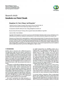
We consider the problem of (progressively) sampling a dense point cloud representation of the Stanford Bunny shown in figure 3. The oversampling of the object is a typical data acquisition result and usually requires data reduction before any kind of surface reconstruction and/or rendering can be attempted. Instead of data reduction, we sample 10

the point cloud using FastFPS for point clouds and render the resulting uniform and adaptive point sets. To apply FastFPS for point clouds to this point set, we embed the

Figure 3: Full resolution representation of Stanford Bunny. surface representation in a 3D Cartesian grid. The FastFPS algorithm is then used to sample the point cloud both (irregularly) uniformly and adaptively following the selection of a starting sample point within the outside offset band surrounding the surface. For simplicity, r was set to a uniform 2∆x. Figure 4 presents both the uniform and adaptive sample point sets produced by FastFPS for sample point budgets of 1.4%, 2.8%, 11.1% and 22.2% of the size of the original point set respectively. The non-uniform point sets were obtained by weighing each surface point by an approximation of the local curvature. From the inspection of figure 4, it is evident that in the non-uniform case, the majority of samples is placed in regions which are relatively less smooth. For the Bunny model and the curvature approximation used here, this leads to relatively poor results for small sample point budgets when compared to the renderings of the corresponding uniform point sets. For larger point budgets, however, non-uniform sampling yields increasingly better results due to the availability of locally dense point samples in areas of relatively high curvature such as the paws. This effect is strengthened when choosing a point-based local importance measure such as Pauly et al [16] “surface variation” measure. 11

5

Conclusions

We presented an extension of the Fast Marching farthest point sampling principle introduced in Moenning and Dodgson [13] to the case of surfaces given in implicit or point cloud form. By making use of a recently proposed extension to the Fast Marching framework [11, 12], this extended FastFPS algorithm retains the computational efficiency and ease of implementation of the basic FastFPS algorithm. The restrictive requirement of (acutely) triangulated domains associated with the basic FastFPS algorithm for surfaces [13] is therefore overcome by the suggested extension and a new implicit surface or point cloud sampling algorithm yielding uniform or adaptive sample point sets is obtained. Possible applications include progressive acquisition, surface encoding and compression, progressive transmission and (progressive) rendering. As regards further FastFPS-related research, we are currently working on detailed comparative studies regarding the quality of FastFPS sample point sets generated from images and surfaces relative to sample point sets produced by relevant alternative sampling strategies. This work includes the analysis of any explicit guarantees which can be made regarding the nature of FastFPS sample point sets. On the application side, we are interested in using uniform FastFPS surface sample point sets alongside subdivision displacement maps [9] for multiresolution surface representations. In the case of point clouds, point-based (multiresolution) representations for pointbased rendering are readily available [1, 10, 17]. With regard to adaptive point cloud sampling, we are investigating point-based curvature approximations yielding results superior to the curvature approximation employed in the previous section. Finally, we are exploring the use of FastFPS as a link between the data acquisition and surface reconstruction/rendering steps in a fully integrated and automated surface processing pipeline [19, 20]. With the help of point-based curvature approximations and FastFPS, previously collected samples may be used for the determination of future sample point locations thereby, for example, concentrating relatively more samples in regions of high curvature.

Acknowledgements The Bunny model was obtained from the Stanford 3D Scanning Repository at http://graphics.stanford.edu/data/3Dscanrep. We have benefited from numerous discussions with Michael Blain, Marc Cardle and Mark Grundland.

References [1] M. Alexa, J. Behr, D. Cohen-Or, S. Fleishman, D. Levin and T. Silva. Point Set Surfaces. Proc. of the 12th IEEE Visualization Conf., San Diego, USA, pages 21–28, 2001. [2] F. Aurenhammer. Voronoi Diagrams - A Survey of a Fundamental Geometric Data Structure. ACM Computing Surveys, 23(3):345–405, 1991. 12

[3] O. Cuisenaire. Distance Transformations: Fast Algorithms and Applications to Medical Image Processing. Ph.D. thesis, Universit´e catholique de Louvain, Laboratoire de Telecommunications et Teledetection, Belgium, 1999. [4] M. Desbrun, M. Meyer, P. Schr¨oder and A. Barr. Discrete-differential operators in nD. California Institute of Technology/USC Report, 2000. [5] Y. Eldar. Irregular Image Sampling Using the Voronoi Diagram. M.Sc. thesis, Technion - IIT , Israel, 1992. [6] Y. Eldar, M. Lindenbaum, M. Porat and Y. Y. Zeevi. The Farthest Point Strategy for Progressive Image Sampling. IEEE Trans. on Image Processing, 6(9):1305–1315, 1997. [7] R. Kimmel and J. A. Sethian. Computing Geodesic Paths on Manifolds. Proc. of the Nat. Acad. of Sciences, 95(15):8431–8435, 1998. [8] R. Kimmel and J. A. Sethian. Fast Voronoi Diagrams and Offsets on Triangulated Surfaces. Proc. of AFA Conf. on Curves and Surfaces, Saint-Malo, France, 1999. [9] A. Lee, H. Moreton and H. Hoppe. Displaced Subdivision Surfaces. Computer Graphics Proc., SIGGRAPH ’00, Annual Conference Series, pages 85–94, 2000. [10] L. Linsen. Point cloud representation. CS Technical Report, University of Karlsruhe, Germany, 2001. [11] F. M´emoli and G. Sapiro. Fast Computation of Weighted Distance Functions and Geodesics on Implicit Hyper-Surfaces. Journal of Computational Physics, 173(1):764– 795, 2001. [12] F. M´emoli and G. Sapiro. Distance Functions and Geodesics on Point Clouds. Technical Report 1902, Institute for Mathematics and its Applications, University of Minnesota, USA, 2002. [13] C. Moenning and N. Dodgson. Fast Marching farthest point sampling. University of Cambridge, Computer Laboratory Technical Report No. 562 , Cambridge, UK, 2003. [14] I. Notkin and C. Gotsman. Parallel progressive ray-tracing. Computer Graphics Forum, 16(1):43–55, 1997. [15] A. Okabe, B. Boots and K. Sugihara. Spatial Tessellations - Concepts and Applications of Voronoi Diagrams. 2nd ed. John Wiley & Sons, Chicester, UK, 2000. [16] M. Pauly, M. Gross and L. P. Kobbelt. Efficient Simplification of Point-Sampled Surfaces. Proc. of the 13th IEEE Visualization Conf., Boston, USA, 2002. [17] H. Pfister, M. Zwicker, J. van Baar and M. Gross. Surfels: Surface Elements as Rendering Primitives. Computer Graphics Proc., SIGGRAPH ’00, Annual Conference Series, pages 335–342, 2000. [18] E. Rouy and A. Tourin. A viscosity solutions approach to shape-from-shading. SIAM Journal of Numerical Analysis, 29(3):867–884, 1992. 13

[19] S. Rusinkiewicz, O. Hall-Holt and M. Levoy. Real-Time 3D Model Acquisition. Computer Graphics Proceedings, SIGGRAPH ’02, Annual Conference Series, pages 438-446, 2002. [20] R. Scopigno, C. Andujar, M. Goesele and H. Lensch. 3D Data Acquisition. EUROGRAPHICS 2002 tutorial , Saarbr¨ ucken, Germany, 2002. [21] R. Sedgewick. Algorithms in C++. 3rd ed. Addison-Wesley, Reading, USA, 1998. [22] J. A. Sethian. A fast marching level set method for monotonically advancing fronts. Proc. of the Nat. Acad. of Sciences, 93(4):1591–1595, 1996. [23] J. A. Sethian. Level Set Methods and Fast Marching Methods - Evolving Interfaces in Computational Geometry, Fluid Mechanics, Computer Vision, and Materials Science. 2nd ed. Cambridge University Press, Cambridge, UK, 1999. [24] J. A. Sethian. Fast Marching Methods. SIAM Review , 41(2):199–235, 1999. [25] M. I. Shamos and D. Hoey. Closest-point problems. Proc. of the 16th Annual IEEE Symp. on Foundations of Computer Science, pages 151–162, 1975. [26] A. P. Witkin and P. S. Heckbert. Using Particles to Sample and Control Implicit Surfaces. Computer Graphics Proc., SIGGRAPH ’94, Annual Conference Series, pages 269–278, 1994. [27] Y. Y. Zeevi and E. Shlomot. Non-uniform sampling and anti-aliasing in image representation. IEEE Trans. on Signal Processing, 41:1223–1236, 1993.

14

Figure 4: Uniform (left) and adaptive (right) point sets produced by FastFPS for implicit surfaces and point clouds for sample budgets of (a) 1.4%, (b) 2.8%, (c) 11.1% and (d) 22.2% of the size of the original point cloud.

15