Fast Neighbor Cells Finding Method for Multiple Octree Representation Jaewoong Kim and Sukhan Lee F
Abstract—A cell occupancy map has been used widely for efficiently representing obstacles in robotic navigation. Such a map can often be formed based on the multi-resolution octree representation (MOR) of 3D point clouds captured from objects and workspace. This elevated cell-based approach may offer the capability of understanding the geometric context of workspace, expanding its applicability to robotic manipulation in a cluttered workspace. Under this context, the main issue of MOR becomes how to represent and generate cell addresses in such a way as to find neighboring cells efficiently. This paper presents a novel method for efficiently searching for neighboring cells with the fast generation of all the neighboring cell addresses. The original contribution of this paper is that not only the direct neighbors defined by those cells the edges or corners of which are directly connected to the given cell, but also the indirect neighbors of distance r, defined by those cells being separated from the given cell by the distance r, are included. The proposed method have been implemented and applied to obstacle representation in the 3D workspace modeling.
T
I.. INTRODUCTION
HE multiple resolution octree representation (MOR), a method of modeling 3D workspace in the form of a cell occupancy map, has been regarded as one of the candidates that best qualify for the criteria stated above[1]. Thank to its simplicity in representation and update, MOR has been settled to date as one of viable platforms for real-time path/motion planning in navigation [2]-[5]. However, as a cell-based representation, MOR has an inherent limitation on its descriptive power for defining objects, walls, obstacles, free space, etc. as distinct entities in 3D workspace. Often, path/motion planning prefers these distinct entities being identified in order to understand the geometric context of 3D workspace, based on which a more globally optimal path/motion could be found. This paper intends to elevate the descriptive power of MOR to the level that such distinct entities as objects, walls, obstacles, free space, etc. can be identified with MOR in real-time. Improving the efficiency This research is performed for the 21st Century Intelligent Robot National Frontier Project sponsored by the Korea Ministry of Knowledge Economy (MKE). This research is also supported in part by the Korea Science and Engineering Foundation (KOSEF) grant sponsored by the Ministry of Education, Science and Technology (MEST), No. R01-2006000-11297-0, and in part by the Science and Technology Program of Gyeonggi Province, and also supported by the MKE(Ministry of Knowledge Economy), Korea, under the ITRC(Information Technology Research Center) support program supervised by the IITA(Institute of Information Technology Advancement) (IITA-2009-(C1090-0902-0046)), Jaewoong Kim and Sukhan Lee*, the Corresponding Author, are with the Intelligent Systems Research Center, Sungkyunkwan University, Suwon, Korea (e-mail:
[email protected] and
[email protected] , respectively).
Fig. 1. Overall Process Diagram
for storing an occupancy map as well as for cell searching and finding the neighboring cells have been investigated based on assigning proper codes to individual MOR cells. A lot of research have been suggested the octree addressing, encoding and searching issue in MOR, because of that can successfully help to provide space, object and map information which used in real-time path/motion planning. So we can find out specific octree cell information in MOR through our advanced octree neighbor finding method. The classical neighbor finding method is proposed by Samet[6]. He suggested to find the neighbor cells in the given direction for pointer octrees based on the search of a common ancestor. Besançon revised the algorithm and suggested the encoding technique[7]. Ballard and Brown[8] suggested the backtracking method in the tree structure, and to find neighbor from initial cell to common ancestor. This method is based on recursive structure of tree and designed to minimize backtracking from logical function to verify the neighboring status between two cells. Vörös. J[9] suggested a matrix based octree finding strategy using locational binary code for repetitive neighbor finding profits from both forms of representation. He start to treat both the same and the difference resolution octrees for neighbor finding. Until a recent date, Payeur P[10] proposed a good method for finding nearest neighbor cells each 26 directions in MOR. Generic neighboring rule set is proposed in the paper, which relies on a hierarchical addressing scheme of cells and a set of algebraic rules encoded as lookup table. The relation between the direction and a rule set of possibility is defined, and used simultaneously when the selected cell meets other cells. In the paper, other validating rules and lookup table in
MOR case are also explained. Nevertheless, the research focus on the direct connected cell finding method that relies on the direction of initial selected cell, the indirect connected cases cannot be explained. And he did not exactly mention about when selected cell located on the boundary of octree structure. It does not frequently occur in his explanation but it cannot cover all place in octree structure when sometime finder bring to wrong result.
(a) Payeur’s address encoding method (b) Our address encoding method Fig. 2. Address encoding methods of the octree structure
II. OVERALL ALGORITHM In Fig 1, we show the our overall process diagram. We introduce our key function for finding the neighbors and address generation. When the octree cell is generated from 3D data acquisition, our algorithm is into it for having a special rule that takes advantage of integer address in the octree structure (Address Encoding). Then we can obtain the sequential rule of the address-encoded address difference value of each octree cell (fADV). Under the rule, we can change form of the selected octree cell address into octree coordinates value (fOCV) with opposite pair of the selected address (fOADV). The octree coordinates value can be used to decide relation of the neighbors between two different octree cells with simple arithmetic decision operation. Additionally, if selected octree cells need to know the address of others around themselves, the octree coordinates value in the same level octree structure is used to calculate the new 26 neighbors address with GCD operation. III. ADDRESS ENCODING IN THE OCTREE COORDINATES The address encoding of the octree structure, that gives address using positive integer of 1 ~ 8 from the origination of back corner of upper left side of octree structure as shown in Fig 2, uses ‘push back’ method that continuously add new integer address value to the last digit of existing address value repetitively increasing digits of address value by octree depth level. A lots of researcher recently use this method because it is easy to understand the information such as depth or location of cell intuitively with just seeing the address value in the case of integer representation. We did not use integer 0 in address value different from other research groups, because 0 is the special meaning number in integer theory and four fundamental rules of arithmetic mainly used in the method suggested by this paper. The Octree Coordinates that 3 axis are relatively orthogonal is defined and shown in Fig 3 so that root cell be the center of gravity to represent what location randomly selected octree cell take in whole structure and to help understanding proposed method. From the origin, x axis is set for left and right direction, y axis for up and down direction and z axis for front and back direction for each and + direction for increasing direction of address, - direction for decreasing in the case of encoding the cell address. The addresses encoded to octree coordinate have characteristics of showing the differences of magnification
Fig. 3. The Octree Coordinates
such as 4 times to y axis from x axis and 2 times to z axis, and this means address sequence rule has the same characteristics irrelevant to axis. IV.THE CHARACTERISTICS OF THE ENCODED ADDRESS Every cell in the generated octree structure will has unique address value for each, when the initial root cell is divided at the certain level with explained method before. There will be address difference value that has unique regularity of series in x, y, z axis; this feature enables us to judge the distance or adjacent relation between cells or to generate addresses. Let’s define these “Address Difference Values” as “ADV”. Encoded address has two major characteristics; (a) ADV additionally chosen to prepare adjacent relation with selected cell must have the value of specific regularity in x, y, z direction of octree coordinates and can be expressed in series or set (b) There must exist 3 cells located vertically opposite side of x-y, y-z, and z-x plane centered by the origin of octree coordinates from the selected cell. We define this as opposite or mirroring pair. A. Characteristics of the ADV Column samples of certain cell are shown with level of 1 to 3 for each x, y, z axis in Fig 4 to explain characteristic (a) above, and all increment/decrement difference values of ADV between adjacent cells under column are marked. In the example of x axis, there is ADV 1 in case of depth level 1, 1 in level 2, 1, 9 and 89 in level 3. There is maximum 2 n-1 ADVs when n is level, maximum number of ADV corresponding to each level is same independent of axis. Y axis and z axis also show same pattern with x axis, and we can find y axis has exact 4 times value of ADV from x value, z axis has 2 times value of ADV as explained earlier. These characteristics can be summarized as Table 1, also can be formulated as equation (1). f ADV X , I = f
{
ADV
X , I −1 8 ∗ a0 ∗ 10 I
0 ≤ I ≤ maximum level of structure a 0 : 1 x axis , 4 y axis , 2 z axis
(1)
(a) address arrays of x axis
(b) address arrays of y axis
(c) address arrays of z axis
Fig 4. Example of address arrays of x, y and z axis. TABLE 1 CHARACTERISTICS OF ADDRESS DIFFERENCE VALUE Digit Index X axis Y axis Z axis 1 0 1 4 2 2 1 9 36 18 3 2 89 356 178 4 3 889 3556 1778 5 4 8889 35556 17778 6 5 88889 355556 177778 7 ... ... ... ... 8 n-1 8....(8)....9 3....(5)....6 1....(7)....8
We can get available ADV any time using the function f ADV in the equation (1) if the level and axis of selected cell structure is determined. B. OADV of Selected Address The address of selected octree cell can be converted to coordinates value presenting the location on octree coordinates using ADV characteristics, these value are useful to understand the direct/indirect adjacent relation between octree cells with various size later. To get coordinate value of selected cell in octree coordinates, the Opposite Pair is needed. The Opposite Pair means a pair of cells located in mutually opposite side based on x-y, y-z and z-x plane centered by the origin of octree coordinates as mentioned in ADV characteristics (b). When one cell address is selected, it brings opposite pairs for each x, y, z and you can easily see in the example shown in level 3 of (a), (b), and (c) in Fig 4. For example, the address of opposite pair is 141 if 232 is chosen to x axis array, 433 for chosen 877 to y axis and 134 for chosen 312 to z axis. This means the cells with mutually same distance is chosen based by 0 of array of each axis. This is also relevant to the characteristic that numbers of 1 to 8 can be shown only from specific direction centered by the origin of octree structure, this characteristic that is recently used by Payeur. P[10] can be summarized as Table 2. Conversion of all digits of address of selected cell to the numbers selected in needed direction of x, y, z axis through Table 2 easily brings opposite pair and also we can easy make it by using the function f OADV from the equation (2). f OADV X , A = ∣ Aopp − A ∣
{
(2) , A : selected address Two cells in opposite pair relation also have one ADV, we regard this value as ADV in special relation and define as OADV (opposite pair’s ADV). OADV can be calculated by Aopp :Opposite Pair Address of Alook up digit in Table 2 X : x,y and z axis
TABLE 2 OPPOSITE DIGIT TABLE X axis Y axis Z axis 2 5 3 1 6 4 4 7 1 3 8 2 6 1 7 5 2 8 8 3 5 7 4 6
deduction of itself from the address in opposite pair relation of selected address, and there is characteristic that all OADV from the selection of array of one axis among x, y, z axis on octree structure with specific level has unique value to the specific axis. We can generalize selected cell address to the octree coordinates value presenting location on octree structure through some arithmetic calculation of OADV using this property. OADV deducted by the maximum value of ADV at corresponding level results integers that begins from 0 and not duplicated, we can observe the property getting binary pattern by dividing this value by twice of initial value in corresponding direction. Conversion of this binary pattern into decimal value results single integer value between 0 and 2n-1 (n is the maximum level value on corresponding octree structure), this value can be used as coordinate value on octree coordinates. This can be formulated as equation (3) based on equation (1) and (2). ∣ f ODAV X , A− A− f ADV X , I max∣ f OCV A = BIN2DEC a0∗2
{
BIN2DEC : Binary to Decimal operation X : x,y and z axis , A : selected address I max : Maximum Index of each axis array
(3)
a 0 : 1 x axis , 4 y axis , 2 z axis
Sign of coordinate value from equation (3) uses the same sign of OADV and one can be generated (total three) for each direction of x, y, z to single selected cell address. These coordinate values are used to calculate the distance between cells or to judge adjacent relation of cells with same or different size using other coordinate value. V. DECISION METHOD OF THE NEIGHBOR IN THE MOR In the case of comparison of randomly selected two cells with different size, there are two cases, (a) one belongs to
any number of elements in the final distance vector of f Dist is lower than desire distance r, then it has a neighborhood relation. The number 1 is the most nearest adjacent cells in all directions when user set the inner boundary distance r equal to 1. Fig. 5. Example of the Decision Method of the Neighbor in the MOR
another, or (b) one keeps a certain distance to another in x, y, z direction. And in the case of two cells with same size, (a) two are identical, or (b) same as (b) above. We can understand the relation between cells intuitively using their coordinate values if the level of targeting two cells is same, can compare by very simple arithmetic which is as following. First, define coordinate values of lower level cell from coordinate values of two cells of different size as OL(xL, yL, zL) and one of higher level as OH(xH, yH, zH), and define the difference between level of two cells as d. And also we can define the compensation value cx,y,z that predefines from the sign of each axis’ OCVs. The compensation value cx,y,z is defined for distinction of same amount number of OCVs in the octree coordinates, it has only 0 and 1 values when the sign of same axis OCV from selected two cells is different and same. We can define as xL-H in the case of comparison for only x among coordinate values. We can also calculate yL-H and zL-H in the same way, this way is the procedure unifying cells of octree structure with two different levels into same level, and xL-H, yL-H and zL-H become the size of difference of two coordinate values after unification of high level. These values can get the distance between two cells by the absolute value of difference the with maximum number of cell, N, that can be virtually generated in case of division of low level cells into high level cells. Calculated indicate inclusion or the distance with the direct comparison with N, that conclusion inside is the case of less than N and distance between cells with the difference with N is the case of same of larger than N. Formulation of this process can be expressed as the function f Dist in the equation (4) below and Fig 5 shows the example. ∣x ∣ ∣x ∣d −1 2 L −1 2 L xH xH cx y y d A = 2∣ L∣−1 − y H 2∣ L∣ −1 − y H 2 c y ∣z ∣ ∣z ∣d −1 zH zH cz 2 L −1 2 L
∣[ ] [ ]∣ ∣[ ] [ ]∣ [ ] f Dist O H , OL =
A − 2 d −1
(4)
2 1 , when selected twoOCVs signis different c x,y,z = 0 , when selected two OCVs sign issame
{
d : Difference value of Level L and H f Dist O H , OL =0 , when f Dist O H , O L ≤0
If we select two cells that have difference value d is 2 as example in the Fig 5, OL1(0, -0, -0) and OH(4, -0, -2), then we can get the final result A is [5 0 3]T and f Dist O H ,O L1 is [1 0 0]T from given function. This result is directly used cell distance between selected two cells, zero number means that has inner bounded or overlapped relation of those cells. If
VI. GENERATION OF 26 ADJACENT ADDRESSES IN THE SAME LEVEL Sometimes we wish to know not just adjacent relation but also address value of adjacent, we suggest the method that generate 26 addresses quickly using 6 ADV from directions of -x, +x, -y, +y, -z and +z based on the address of selected cell with the same level and their combination. Generally selected octree cell excluding octree located at boundary surface and vertex has nearest neighbor cell through 6 planes, 12 boundary lines and 8 vertexes. ADVs interfacing with 6 planes by proposing method are essential so it should be calculated before other adjacent ADVs. Octree Coordinate values that is made through OADV of cell address selected with previously explained method have special relation with the maximum number of cells that the level of corresponding octree structure can have as one column or row, this special property is Greatest Common Digit (GCD) relation. GCD value with 1 and multiples of 2 can be calculated by GCD calculation between two numbers, and the multiplier that represents this value as multiplication of 2 shows the same meaning of what order of factors should be selected in ADV series shown in Table 1. Table 3 shows ADV distribution with one column from x axis on octree structure with level 4 and example of GCD value, for example selection of address value 1141 results final GCD value 1 in Table 4. 1 is 20, so the first(first index) ADV value to x axis indicates the first factor value 1 in series as shown in Table 1. Because the sign of OADV is positive, it indicates ADV value in direction of +x that value finally becomes 1. To calculate the opposite direction ADV, we can use ADV value of other adjacent cell in original direction. For example, we can find out that ADV of 1141 in –x direction is same as ADV of 1132 in +x direction. To get this value, GCD calculation between OADV of 1132 and the maximum number of cells is expected; however GCD calculation between coordinate value of adding 1 to the coordinate value of 1141 and the maximum number of cells brings results without additional calculation. We can get GCD value 2 as results, can select the second factor 9 indicated by 1 of x axis in Table 1 because 2 are 21. The sign of ADV is negative because of opposite direction. Coordinate value has the extremal value for the case of cell which coordinate value belongs to border; no calculation is needed because any ADV can exist in – direction for positive OADV, and + direction for negative OADV. ADV in 6 direction made with this way can generate adjacent address in addition to selected cell address at once. 12 neighborhood adjacent with the line as in Fig 6 can generate new ADV made from 12 combination that can
TABLE 3 EXAMPLE OF ADV DISTRIBUTION WITH ONE COLUMN FROM X AXIS ON OCTREE STRUCTURE WITH LEVEL 4 ADDR OPP SIGN OCV GCD (-)ADV (+)ADV 1131 2242 7 1 1 1132 2241 6 2 -1 9 1141 2232 5 1 -9 1 1142 2231 4 4 -1 89 + 1231 2142 3 1 -89 1 1232 2141 2 2 -1 9 1241 2132 1 1 -9 1 1242 2131 0 8 -1 889 2131 1242 0 8 -889 1 2132 1241 1 1 -1 9 2141 1232 2 2 -9 1 2142 1231 3 1 -1 89 2231 1142 4 4 -89 1 2232 1141 5 1 -1 9 2241 1132 6 2 -9 1 2242 1131 7 1 -1 ADDR: SELECTED OCTREE ADDRESS, OPP: OPPOSITE PAIR OF SELECTED ADDRESS, SIGN: SIGN OF OADV, OCV: OCTREE COORDINATES VALUE, GCD: GREATEST COMMON DIGIT OF BOTH OCV AND 23, (-)ADV : ADV OF –X DIRECTION, (+)ADV : ADV OF +X DIRECTION
chose 2 without duplication excluding same axis in 6 directions, remaining neighborhood adjacent with 8 vertex can be found by addition of ADVs from 8 combination that can chose 3 from 6 without duplication. VII.EXPERIMENTS & RESULTS MOR can be used to represent objects and obstacles placed in 3-dimensional space and can be effectively used to robot navigation or routing plan of robot arm. As one clear application, we will show that our research can be excellently applied to 3D Workspace modeling (3DWM) written by Sukhan Lee’s research[3] through our experiment. Based on Lee’s research, 3-dimensional environment for robot arm doing tasks is defined as ‘Workspace’ and working environment is interpreted using stereo camera. Existence of object is presented by MOR dividing 3dimensional point clouds gained by stereo camera from root cell to specific level; this result is used as the presentation of obstacles in workspace or routing plan of robot arm. There was a problem that much calculation is needed to interpret relations about all generated octree cell because one octree cell is considered as one object in the past researches, while existing one mass of object is shown by multiple octree cell this time. Proposed method shows to effectively decrease in calculation by supporting multiple various sized octree cell presented as one object with applying addresses to multiple octree cell generated and clustering to solve this problem. We use the Intel(R) Core(TM)2 Duo 2 2.40Ghz processor, and 2Gbytes memory. We perform our experiment based on the VC++ .net. Framework 2.0 compiler. We set the 3DWM experiment environments in Fig. 7, and from Fig 8 to Fig 10, we also shows the openGL rendering results of 3DWM that contain the 3D point clouds, table and clustered octree cells. We take two experiments in the 3DWM(in the Fig 9 and
Fig. 6. Example of the relation among 26 nearest neighbor ADVs
10) for comparing of various algorithm performances that is our method, Payuer’s method and general backtracking method, and for reasonable results, we performed over the 100 times same iteration process per each experiment. In Table 4 we can show the final performance results of two experiments. And we also show the detail openGL rendering results of the octree clustering in Fig 9 and Fig 10. Follow the Table 4 we can reduce a lots of waste time for finding neighbors in MOR successfully. The proposed algorithm complexity depends on the number of resolution levels in MOR because the encoding process from arithmetic operation and GCD calculation cannot avoid the problems. Finding the nearest neighbor, i.e. the direct contact cells, one cell selected and the other cell arrived together with direction information for comparing each other in MOR. The maximum complexity of Payuer’s method[10] is O(p-1), Gargantini’s method[8] is O(p) and classical backtracking method is O(23(p-1)) where p represents the maximum number of resolution levels in MOR. However if the direction information is unknown, at most 26 times iteration are needed to find neighbor and generate address. In that case, the Payuer’s maximum complexity is O(26(p-1)) when there is no direction information given. But the complexity of our method in the same condition is O(6(p-1)), only a quarter of the former one. Because of the arithmetic operation time does not require complexity. In indirect connected neighbor finding case, other approaches depend on the distance for finding in MOR, because of the fact that they only regard the direct connected case. So their maximum complexity will be changed O((p-1)r) where r represents the maximum distance. But our proposed method does not need to change the order, because at most 6 order need to obtain the location information in MOR. VIII.CONCLUSION In this paper we proposed simple and fast neighbor finding method that uses simple arithmetic and GCD operation instead of searching with complex hash table table or direction information. It is an efficient way to understand clusters in 3D space. It can contribute for searching direct and indirect(within any distance) neighbor relation between
TABLE 4 EXPERIMENT RESULTS OF OCTREE CLUSTERING IN THE OCTREE STRUCTURE EXPERIMENT #1 Lv1
Lv2
Lv3
Lv4
Lv5
Lv6
Lv7
Lv8
Lv9
Total
M1
M2
Level 6
0
0
0
0
1
78
0
0
0
79
0
0
94
Level 7
0
0
0
0
1
11
200
0
0
212
0
47
781
Level 8
0
0
0
0
1
11
30
405
0
447
0
172
4094
Level 9
0
0
0
0
1
41
996
1079
16
1015
29094
11 30 EXPERIMENT #2
M3
Lv1
Lv2
Lv3
Lv4
Lv5
Lv6
Lv7
Lv8
Lv9
Total
M1
M2
M3
Level 6
0
0
0
0
1
132
0
0
0
113
0
15
250
Level 7
0
0
0
0
1
12
336
0
0
349
0
94
2110
Level 8
0
0
0
0
1
12
34
906
0
953
0
734
18813
0 0 0 0 1 12 34 102 2221 2370 62 4812 N/A LV #: AMOUNT OF GENERATED OCTREE CELLS IN THE EACH LEVEL #, TOTAL: TOTAL AMOUNT OF GENERATED OCTREE CELLS, M1: PROPOSED METHOD & PROCESSING TIME (MSEC), M2: PAYEUR’S METHOD & PROCESSING TIME (MSEC), M3: GENERAL BACKTRACKING METHOD & PROCESSING TIME (MSEC) Level 9
Fig. 7. Experiment Environments of 3D Workspace Modeling
Fig. 9. The octree clustering result of Experiment #1 (Level 9)
two different cells in 3-Dimensional vector space, robot path planning, visualization and modeling. For future we will keep up with the evaluated our method within constant time algorithm for better performance. REFERENCES [1] [2] [3]
[4]
Dana H. Ballard and Christopher M. Brown, “Computer Vision,” PRENTICE HALL, 1982. M. A. Garcia and A. Solana, “3D Simultaneous localization and modeling from stereo vision,” International Conference on Robotics & Automation (ICRA’04), New Orleans, LA, April 2004 Sukhan Lee, Daesik Jang, Eunyoung Kim, Suyeon Hong, and JungHyun Han, "A real-time 3D workspace modeling with stereo camera," Intelligent Robots and Systems, 2005. (IROS 2005). 2005 IEEE/RSJ International Conference on Page(s):2140 – 2147, 2-6 Aug. 2005. Han-Young Jang, Moradi. H, Lee. S, and JungHyun Han, "A visibility-based accessibility analysis of the grasp points for real-time
Fig. 8. The octree clustering result in MOR of 3D Workspace Modeling
Fig. 10 The octree clustering result of Experiment #2 (Level 9) manipulation," Intelligent Robots and Systems, 2005. (IROS 2005). 2005 IEEE/RSJ International Conference on 2-6 Aug. 2005 Page(s):3111 - 3116 [5] Han-Young Jang, Hadi Moradi, Suyeon Hong, Sukhan Lee, and JungHyun Han, "Spatial Reasoning for Real-time Robotic Manipulation," Intelligent Robots and Systems, 2006 IEEE/RSJ International Conference on Oct. 2006 Page(s):2632 - 2637 [6] H. Samet The Design and Analysis of Spatial Data Structures Reading, MA: Addison-Wesley, 1990. [7] J. E. Besançon, Vision par Ordinateur en Deux et Trois Dimensions. Paris, France: Eyrolles, 1988, pp. 341–353. [8] I. Gargantini, Linear oct-trees for fast processing of three-dimensional objects, Computer Graphics and Image Processing 20 (1982) 365– 374. [9] Vörös. J, "A strategy for repetitive neighbor finding in octree representations," Image and vision computing,2000,18(14): pp. 1085– 1091 [10] Payeur, P., "An Optimized Computational Technique for Free Space Localization in Probabilistic Environment Models", IEEE Transactions on Instrumentation and Measurement, vol. 55, no 5, pp. 1734-1746, October 2006.