Fast Algorithms for Finding O(Congestion+Dilation). Packet Routing Schedules. F. T. Leighton. Bruce M. Maggs. Andr ea W. Richa. July 1996. CMU-CS-96-152.
Fast Algorithms for Finding O(Congestion+Dilation) Packet Routing Schedules F. T. Leighton�
Bruce M. Maggs July 1996
Andr�ea W. Richa
CMU-CS-96-152
School of Computer Science Carnegie Mellon University Pittsburgh, PA 15213 Mathematics Department, and Laboratory for Computer Science Massachusetts Institute of Technology Cambridge, MA 02139 �
Abstract In 1988, Leighton, Maggs, and Rao showed that for any network and any set of packets whose paths through the network are xed and edge-simple, there exists a schedule for routing the packets to their destinations in O(c + d) steps using constant-size queues, where c is the congestion of the paths in the network, and d is the length of the longest path. The proof, however, used the Lov�asz Local Lemma and was not constructive. In this paper, we show how to nd such a schedule in O(P (loglog P ) log P ) time, with probability 1 1=P , for any positive constant , where P is the sum of the lengths of the paths taken by the packets in the network. We also show how to parallelize the algorithm so that it runs in NC. The method that we use to construct the schedules is based on the algorithmic form of the Lov�asz Local Lemma discovered by Beck. Tom Leighton is supported in part by ARPA Contracts N00014-91-J-1698 and N00014-92-J-1799. Bruce Maggs and Andr�ea Richa are supported in part by ARPA Contract F33615-93-1-1330 and in part by an NSF National Young Investigator Award, No. CCR-9457766, with matching funds provided by NEC Research Institute. The views and conclusions contained in this document are those of the authors and should not be interpreted as representing the o�cial policies, either expressed or implied, of ARPA, NSF, or the U.S. government.
Keywords: Store and forward networks, Network problems, Network protocols, Combinatorial algo-
rithms
1 Introduction
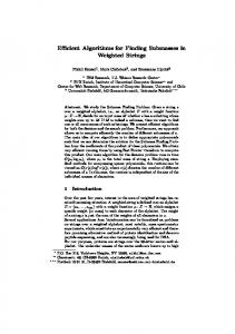
In this paper, we consider the problem of scheduling the movements of packets whose paths through a network have already been determined. The problem is formalized as follows. We are given a network with n nodes (switches) and m edges (channels). Each node can serve as the source or destination of an arbitrary number of messages. Each message consists of an arbitrary number of packets (or cells or its , as they are sometimes referred to). Let N denote the total number of packets to be routed. (In a dynamic setting, N would denote the rate at which packets enter the network. For simplicity, we will consider a static scenario in which a total of N packets are to be routed through the network.) The goal is to route the N packets from their origins to their destinations via a series of synchronized time steps, where at each step at most one packet can traverse each edge. Figure 1 shows a 5-node network in which one packet is to be routed to each node. The shaded nodes in the gure represent switches, and the edges between the nodes represent channels. A packet is depicted as a square box containing the label of its destination. During the routing, packets wait in three di�erent kinds of queues. Before the routing begins, packets are stored at their origins in special initial queues. When a packet traverses an edge, it enters the edge queue at the end of that edge. A packet can traverse an edge only if at the beginning of the step, the edge queue at the end of that edge is not full. Upon traversing the last edge on its path, a packet is removed from the edge queue and placed in a special nal queue at its destination. In Figure 1, all of the packets reside in initial queues. For example, packets 4 and 5 are stored in the initial queue at node 1. In this example, each edge queue is empty, but has the capacity to hold two packets. Final queues are not shown in the gure. Independent of the routing algorithm used, the size of the initial and nal queues are determined by the particular packet routing problem to be solved. Thus, any bound on the maximum queue size required by a routing algorithm refers only to the edge queues. This paper focuses on the problem of timing the movements of the packets along their paths. A schedule for a set of packets speci es which move and which wait at each time step. Given any underlying network, and any selection of paths for the packets, our goal is to produce a schedule for the packets that minimizes the total time and the maximum queue size needed to route all of the packets to their destinations. We would also like to ensure that any two packets traveling along the same path to the same destination always proceed in order. Of course, there is a strong correlation between the time required to route the packets and the selection of the paths. In particular, the maximum distance, d, traveled by any packet is always a lower bound on the time. We call this distance the dilation of the paths. Similarly, the largest number of packets that must traverse a single edge during the entire course of the routing is a lower bound. We call this number the congestion , c, of the paths. Figure 2 shows a set of paths for the packets of Figure 1 with dilation 3 and congestion 3.
1.1 Previous and related work
Given any set of paths with congestion c and dilation d, in any network, it is straightforward to route all of the packets to their destinations in cd steps using queues of size c at each edge. In this case the queues are big enough that a packet can never be delayed by a full queue in front, so each packet can be delayed at most c 1 steps at each of at most d edges on the way to its destination. In [9], Leighton, Maggs, and Rao showed that there are much better schedules. In particular, they established the existence of a schedule using O(c + d) steps and constant-size queues at every edge, thereby achieving the naive lower bounds for any routing problem. The result is highly robust in the sense that it works for any set of edge-simple paths and any underlying network. (A� priori, it would be easy to imagine that there might be some set of paths on some network that required more than (c + d) steps or larger than constant-size queues to route all the packets.) The method that they used to show the existence of optimal schedules, however, is not constructive. In other words, the fastest known algorithms for producing schedules of length O(c + d) with constant-size edge queues require time that is exponential in the number of packets. For the class of leveled networks, Leighton, Maggs, Ranade, and Rao [8] showed that there is a simple on-line randomized algorithm for routing the packets to their destinations within O(c + L + log N) steps, 1
5
4
1
2
3 1
4
5
2
3
Figure 1: A graph model for packet routing. with high probability, where L is the number of levels in the network, and N is the total number of packets. (In a leveled network with L levels, each node is labeled with a level number between 0 and L 1, and every edge that has its tail on level i has its head on level i + 1, for 0 � i < L 1.) Mansour and Patt-Shamir [10] then showed that if packets are routed greedily on shortest paths, then all of the packets reach their destinations within d +N steps, where N is the total number of packets. These schedules may be much longer than optimal, however, because N may be much larger than c. Recently Meyer auf der Heide and Vocking [11] devised a simple on-line randomized algorithm that routes all packets to their destinations in O(c + d + logN) steps, with high probability, provided that the paths taken by the packets are short-cut free (e.g., shortest paths).
1.2 Our results
In this paper, we show how to produce schedules of length O(c + d) in O(P (log log P ) log P ) time, with probability at least 1 1=P , for any constant > 0, where P is the sum of the lengths of the paths taken by the packets. The schedules can also be found in polylogarithmic time on a parallel computer using O(P (log log P ) log P ) work, with probability at least 1 1=P . The algorithm for producing the schedules is based on an algorithmic form of the Lov�asz Local Lemma (see [6] or [13, pp. 57{58]) discovered by Beck [3]. Showing how to modify Beck's arguments so that they can be applied to scheduling problems is the main contribution of the paper. Once this is done, the construction of optimal routing schedules is accomplished using the methods of [9]. The result has several applications. For example, if a particular routing problem is to be performed many times over, then it may be feasible to compute the optimal schedule once using global control. This situation arises in network emulation problems. Typically, a guest network G is emulated by a host network H by embedding G into H. (For a more complete discussion of emulations and embeddings, see [7].) An embedding maps nodes of G to nodes of H, and edges of G to paths in H. There are three important measures of an embedding: the load, congestion, and dilation. The load of an embedding is the maximum number of nodes of G that are mapped to any one node of H. The congestion is the maximum number of paths corresponding to edges of G that use any one edge of H. The dilation is the length of the longest path. Let l, c, and d denote the load, congestion, and dilation of the embedding. Once G has been embedded in H, H can emulate G in a step-by-step fashion. Each node of H rst emulates the local computations performed by the l (or fewer) nodes mapped to it. This takes O(l) time. Then for each packet sent along an edge of G, H sends a packet along the corresponding path in the embedding. The algorithm described in this paper can be used to produce a schedule in which the packets are routed to their destinations in O(c + d) steps. Thus, H can emulate each step of G in O(l + c + d) steps. The result also has applications to job-shop scheduling. In particular, consider a scheduling problem with 2
5
1
4
2
3 1 5
4
2
3
Figure 2: A set of paths for the packets with dilation d = 3 and congestion c = 3. jobs j ; : : :; jr , and machines m ; : : :; ms , for which each job must be performed on a speci ed sequence of machines. In this application, we assume that each job occupies each machine that works on it for a unit of time, and that no machine has to work on any job more than once. Of course, the jobs correspond to packets, and the machines correspond to edges in the packet routing problem. Hence, we can de ne the dilation of the scheduling problem to be the maximum number of machines that must work on any job, and the congestion to be the maximum number of jobs that have to be run on any machine. As a consequence of the packet routing result, we know that any scheduling problem can be solved in O(c+d) steps. In addition, we know that there is a schedule for which each job waits at most O(c + d) steps before it starts running, and that each job waits at most a constant number of steps in between consecutive machines. The queue of jobs waiting for any machine will also always be at most a constant. 1
1
1.3 Outline
The remainder of the paper is divided into sections as follows. In Section 2, we give a very brief overview of the non-constructive proof in [9]. Also we introduce some de nitions, and present two important lemmas which will be of later use. In Section 3, we describe how to make the non-constructive method in [9] constructive, and analyze its running time. In Section 4, we show how to parallelize the scheduling algorithm. We conclude with some remarks in Section 5.
2 Preliminaries In [9], Leighton, Maggs, and Rao proved that for any set of packets whose paths are edge-simple and have congestion c and dilation d, there is a schedule of length O(c + d) in which at most one packet traverses each edge of the network at each step, and at most a constant number of packets wait in each queue at each step. Note that there are no restrictions on the size, topology, or degree of the network or on the number of packets. The strategy for constructing an e�cient schedule is to make a succession of re nements to the \greedy" schedule, S , in which each packet moves at every step until it reaches its nal destination. This initial schedule is as short as possible; its length is only d. Unfortunately, as many as c packets may use an edge at a single time step in S , whereas in the nal schedule at most one packet is allowed to use an edge at each step. Each re nement will bring us closer to meeting this requirement. 1
0
0
1
An edge-simple path uses no edge more than once.
3
The proof uses the Lov�asz Local Lemma ([6] or [13, pp. 57{58]) at each re nement step. Given a set of \bad" events in a probability space, the lemma provides a simple inequality which, when satis ed, guarantees that with probability greater than zero, no bad event occurs. The inequality relates the probability that each bad event occurs with the dependence among them. A set of events A ; A ; : : :; Am in a probability space has dependence at most b if every event is mutually independent of some set of m b 1 other bad events. The lemma is non-constructive; for a discrete probability space, it shows only that there exists some elementary outcome that is not in any bad event. 1
2
Lemma [Lov�asz] Let A ; A ; : : :; Am be a set of \bad" events, each occurring with probability p with depen1
2
dence at most b. If 4pb < 1, then with probability greater than zero, no bad event occurs.
Before proceeding, we need to introduce some notation. A T -frame is a sequence of T consecutive time steps. The frame congestion, Cf , in a T -frame is the largest number of packets that traverse any edge in the frame. The relative congestion, R, in a T-frame is the ratio Cf =T of the congestion in the frame to the size of the frame.
2.1 A pair of tools for later use
In this section we re-state Lemma 3.5 of [9] and we prove Proposition 3.6, which replaces Lemma 3.6 of [9]. Both will be used in the proofs through Section 3.
Lemma 3.5 [9] In any schedule, if the number of packets that use a particular edge g in any y-frame is at most Ry, for all y between T and 2T 1, then the number of packets that use g in any y-frame is at most Ry, for all y � T . Proof: Consider a frame � of size T 0, where T 0 > 2T 1. The rst (bT 0 =T c 1)T steps of the frame can be broken into T -frames. In each of these frames, at most RT packets use g. The remainder of the T 0 -frame � consists of a single y-frame, where T � y � 2T 1, in which at most Ry packets use g. The following proposition will be used in place of Lemma 3.6 of [9].
Proposition 3.6 Suppose that there are positive constants � ; � , � � � , and �, such that in a schedule 1
2
1
2
of size I � (or smaller) the relative congestion is at most � in frames of size I � or larger, and let q be the number of edges traversed by the packets in this schedule. Furthermore, suppose that each packet is assigned a delay chosen randomly, independently, and uniformly from the range [0; I � ] and that if a packet is assigned a delay of x, then x delays are inserted in the rst I � steps of the schedule and I � x delays are inserted in the last I � steps, where � is also a positive constant. Then for any constant � > 0, with probability at least 1 q=I � the relative congestion in any frame of size log I or larger pin-between the rst and last I � steps in the new schedule is at most �(1 + �), for some positive � = O(1)= logI . 1
2
2
3
3
2
3
2
3
Proof: To bound the relative congestion in frames of size log I or larger, we need to consider all q edges 2
and, by Lemma 3.5, all frames of size between log I and (2 log I) 1. As we shall see, the number of packets that use an edge g during a particular T-frame � has a binomial distribution. In the new schedule, a packet can use g during � only if in the original schedule it used g during � or during one of the I � steps before the start of �. Since the relative congestion in any frame of size I � or greater in the original schedule is at most �, there are at most �(I � + T ) such packets. The probability that an individual packet that could use g during � actually does so is at most T=I � . Thus, the probability p that �0 or more packets use an edge g during a particular T frame � is at most 2
2
2
2
2
2
p�
�2 T � � IX (
+
k �
= 0
)
� �(I � + T)� � T �k �1 T �� I T k : k I� I� (
2
2
2+
)
2
To estimate the area under the tails of this binomial distribution, we use the following Cherno�-type bound [5]. Suppose that there are x independent Bernoulli trials, each of which is successful with probability 4
p0 . Let S denote the number of successes in the x trials, and let � = E[S] = xp0. Following Angluin and Valiant [2], we have Pr[S � (1 + )�] � e �= 2
3
for 0 � � 1. p In our application, x = �(I � + T), p0 = T=I � , and � = �(I � + T)T=I � . For = � 3k = logI� (where I � k is any positive constant), � � 1, and T � log I, we have Pr[S �p(1 + )�] � e k � I T T= I k I k I k 0 � � e � e p = 1=I . Setting � T =p (1 + )� = (1 + 3k = logI)�(I + T)T=I , we have �0 � �(1 + k = log I), sinceplog I=I � � 1= logI, for I large enough, for some constant k > 0 (that depends on k ). Let � = k = log I. Then �0 � �(1 + �). Thus p = Pr[S � �0 T ] � Pr[S � (1 + )�] � 1=I k . Since there are at most (I � + I � ) � 2I � starting points for a frame, and log I di�erent size frames starting at each point, and there are at most q distinct edges per frame, the probability that the relative congestion is more than �0 in any frame is at most q2I � log I=I k � q=I k � (for I � 1, 2 log I � I ). Setting k = � + � + 2 completes the proof. 2
2
2
2
2
0 (
0
0 log
0 ln
0
0
2
2
1
0
0
)
2 log
(
)
2
1
0
1
1
2
2
1
1
0
2
2+
2
0
0
1
2
2
2
1
3 An algorithm for constructing optimal schedules In this section, we describe the key ideas required to make the non-constructive proof of [9] constructive. There are many details in that proof, but changes are required only where the Lov�asz Local Lemma is used, in Lemmas 3.2, 3.7 and 3.9 of [9]. The non-constructive proof showed that a schedule can be modi ed by assigning delays to the packets in such a way that in the new schedule the relative congestion can be bounded in much smaller frames than in the old schedule. In this paper, we show how to nd the assignment of delays quickly. We will not regurgitate the entire proof in [9], but only reprove those lemmas, trying to state the replacement propositions in a way as close as possible to the original lemmas. In Section 3.1, we provide a proposition, Proposition 3.2, that is a constructive version of Lemma 3.2 of [9]. In Sections 3.2 and 3.3, we provide three propositions that are meant to replace Lemma 3.7 of [9]. Lemma 3.7 is applied O(log� (c + d)) times in [9]. In this paper we will use Propositions 3.7.1 and 3.7.2 to replace the rst two applications of Lemma 3.7. The remaining applications will be replaced by Proposition 3.7.3. In Section 3.4, we present the three replacement propositions for Lemma 3.9 of [9]. Our belief is that a reader who understands the structure of the proof in [9] and the propositions in this paper can easily see how to make the original proof constructive. Finally, we analyze the running time of our algorithm in Section 3.5.
3.1 The rst reduction in frame size
For a given set of N packets, let c and d denote the congestion and the dilation of the paths taken by these packets, and let P denote the sum of the length of these paths. Let m be the number of edges traversed by the packets (we can ignore the edges not traversed by any packet in the network). Note that m � P � mc. The following proposition is meant to replace Lemma 3.2 of [9]. It is used just once in the proof, to reduce the frame size from d to log P .
Proposition 3.2 For any constant > 0, there is a constant � > 0, such that there exists an algorithm that constructs a schedule of length d + �c in which packets never wait in edge queues and in which the relative congestion in any frame of size log P or larger is at most 1. The algorithm runs in time at most O(P ), and succeeds with probability at least 1 1=P . Proof: The algorithm is simple: assign each packet an initial delay that is chosen randomly, independently,
and uniformly from the range [0; �c], where � is a constant that will be speci ed later. The packet will wait out its initial delay and then travel to its destination without stopping. The length of the new schedule is at most �c + d. Constructing the new schedule takes time at most O(P ). To bound the relative congestion in frames of size log P or larger, we need to consider all m edges and, by Lemma 3.5, all frames of size between log P and 2 log P 1. For any particular edge g, and T -frame �, 5
where log P � T � 2 log P 1, the probability, p, that more than T packets use g in � is at most �c k c � c � � T �k � X T p � 1 �c �c k T k � � � �T T � Tc �c � �T � �e since each of the at most c packets that pass through g has probability at most T=�c of using g in �. (Note that e denotes the base of the natural logarithm.) The total number of frames to consider is at most (�c + d) log P , since there are at most �c + d places for a frame to start, and log P frame sizes. Thus the probability that the relative congestion is too large for any frame of size log P or larger is at most � � P : m log P (�c + d) �e Using the inequalities P � c, P � m; and P � d, we have that for any constant > 0, there exists a constant � > 0, such that this probability is at most 1=P . Before applying Proposition 3.7.1, we rst apply Proposition 3.2 to produce a schedule S of length O(c + d) in which the relative congestion in any frame of size log P or larger is at most 1. For any positive constant , this step succeeds with probability at least 1 1=P . If it fails, we simply try again. =
log
1
3.2 A randomized algorithm to reduce the frame size
In this section, we prove two very similar propositions, Propositions 3.7.1 and 3.7.2, that are meant to replace the rst two applications of Lemma 3.7 of [9], which we state below. Let I � 0. We break a schedule S into blocks of 2I + 2I I consecutive time steps. 3
2
Lemma 3.7 [9] In a block of size 2I + 2I I , let the relative congestion in any frame of size I or greater be at most r, where 1 � r � I . Then there is a way of assigning delays to the packets so that in-between the rst and the last I steps of this block, thep relative congestion in any frame of size I = log I or greater is at most r = r(1 + � ), where � = O(1)= log I . 3
2
2
2
1
1
1
1
After applying Proposition 3.2 to reduce the frame size from d to log P , Proposition 3.7.1 is used to reduce the frame size from log P to (log log P ) , and then Proposition 3.7.2 is used to reduce the frame size from (log log P ) to log ((log log P ) ) = (loglog log P )O . Unlike Lemma 3.7 of [9], Propositions 3.7.1 and 3.7.2 may increase the relative congestion by a constant factor. In general, we cannot a�ord to pay a constant factor at each of the O(log� (c + d)) applications of Lemma 3.7 of [9], but we can a�ord to pay it twice. For the application of Proposition 3.7.1, I = log P and r = 1. With probability at least 1 1=P , for any constant > 0, we succeed in producing a schedule, S , in which the relative congestion is at most O(1) in frames of size log I = (log log P ) (if we should fail, we simply try again). In the application of Proposition 3.7.2, I = (log log P ) , and r = O(1). In the resulting schedule, S , the relative congestion is at most O(1) in frames of size log ((log log P ) ) = (log loglog P )O , with probability at least 1 1=P , for any constant > 0. At this point, we start using Proposition 3.7.3. 2
2
2
2
(1)
2
2
2
2
2
3
2
(1)
Proposition 3.7.1 Let the relative congestion in any frame of size I or greater be at most r in a block of size 2I + 2I I , where 1 � r � I and I = log P . Let Q be the sum of the lengths of the paths taken by 3
2
the packets within this block. Then there is an algorithm for assigning initial delays in the range [0; I] to the packets so that in-between the rst and last I steps of the block, theprelative congestion in any frame of size log I or greater is at most 2r0, where r0 = r(1 + �) and � = O(1)= logI . For any constant > 0, the algorithm runs in time at most O(Q(log log P ) log P ), with probability at least 1 1=P . 2
2
Proof: We de ne the bad event for each edge g in the network and each T-frame �, where log I � T � 2
2 log I 2
1, as the event that more than r0T packets use g in �. A particular bad event may or may not 6
occur, i.e. may or may not be true, in a given schedule. If no bad event occurs, then by Lemma 3.5, the
relative congestion in all frames of size log I or greater will be at most r0. Since there are log I di�erent frame sizes and there are at most (2I + 2I I) + I = 2I + 2I di�erent frames of any particular size, the total number of bad events involving any one edge is at most (2I + 2I ) log I < I , for I greater than some large enough constant. We now describe the algorithm for nding the assignment. We process the packets one at a time. To each packet, we assign a delay chosen randomly, independently, and uniformly from 0 to I. We then examine every event in which the packet participates. We say that the event for an edge g and a T-frame � is critical if delays have p been assigned to C packets that could possibly use g in �, and, of these, more than CT=I +kr(I +T )T=(I log I) packets actually use g during �, where k is a positive constant (to be speci ed later). Intuitively, the event becomes critical if the number of packets assigned delays so far thatptraverse edge g in � exceeds the expected number of such packets (CT=I) by an excess term kr(I + T )T=(I log I), which is the maximum nal excess with respect to the nal expected value that we allow. Note that C � r(T + I). If a packet causes an event to become critical, then we set aside all of the other packets that could also use g during �, but whose delays have not yet been assigned. Let P denote the set of packets that are assigned delays. We will deal with the packets that have been set aside later. As we shall see, after one pass of assigning random delays to the packets, the problem of scheduling the packets that have been set aside is broken into a collection of much smaller subproblems, with probability at least 1 1=P , for any constant 0 > 0. In a pass, we assign a random delay to each packet, and check whether the event for edge g and T -frame � becomes critical. We can do this checking as we construct the schedule in a per time step fashion. When considering time t, we compute the number of packets that traverse each edge g used during t and then we compute the frame congestion of the T -frames ending at t, for T 2 [log I; 2 log I 1]. Note that the frame congestion of the T-frame ending at time t can be computed by taking the frame congestion of the T-frame ending at t 1, subtracting the occurrences of edges in time t T and adding the occurrences of edges in time t. This can be done in time O(Q log I) � O(Q(log log P ) ), Q being the sum of the number of edges in the paths taken by the packets within the block. In the remaining of this paper, we assume we check for the congestions of all T-frames of a block, log I � T < 2 log I, as just described. If a pass fails to reduce the component size, we try again. Since a total of at most r(I + T) packets that traverse edge g have been assignedp delays, the relative � r(1 + congestion for theppackets in � due to the ppackets in P is at most [rT(I + T)(1 + k= logI)=I]=T p p 1= log I)(1 + k= log I) � r[1 + (2k + 1)= log I], since T < 2 log I and 2 log I=I � 1= log I, for I large enough. Choose k so that the relative congestion due to the packets in P in � is at most r0 = r(1 + �). In order to proceed, we must introduce some notation. Let m0 be the number of edges traversed by some packet within the block. The dependence graph, G, is the graph in which there is a node for each bad event, and an edge between two nodes if the corresponding events share a packet. Let b denote the degree of G. Whether or not a bad event for an edge g and a time frame � occurs depends solely on the assignment of delays to the packets that pass through g. Thus, the bad event for an edge g and a time frame � and the bad event for an edge g0 and a time frame � 0 are dependent only if g and g0 share a packet. Since at most r(2I + 2I I) � rI packets pass through g, and each of these packets passes through at most 2I + 2I I � I other edges g0 , and there are at most I time frames � 0, for I large enough, the dependence b is at most rI . For r � I, we have b � I . Since the packets use at most m0 di�erent edges in the network, and for each edge there are at most I bad events, the total number of nodes in G is at most m0 I . We say that a node in G is critical if the corresponding event is critical. We say that a node is endangered if its event shares a packet with an event that is critical. Let G denote the subgraph of G consisting of the critical and endangered nodes and the edges between them. If a node is not in G , then all of the packets that use the corresponding edge have already been assigned a delay (and since this event is not critical, the relative congestion on this edge in the corresponding time frame is at most r0 T), and the bad event represented by that node cannot occur, no matter how we assign delays to the packets not in P . Hence, from here on we need only consider the nodes in G . We are going to show that, with high probability, the size of the largest connected component U of G is at most I log P . Since di�erent components are not connected by edges in G , no two components share a packet. Also any two events that involve edges traversed by the same packet share an edge in G , and so 2
3
2
2
3
2
3
2
2
4
0
2
2
2
2
2
2
3
3
2
2
2
2
4
4
4
12
13
4
4
1
1
1
1
52
1
1
7
are in the same connected component. Thus there exists a one-to-one correspondence between components of G and disjoint sets in a partition of the packets not in P. Hence, we can assign the delays to the packets in each component separately, and we have reduced the size of a largest component in G from m0 I to I log P . The trick to bounding the size of the largest connected component U is to observe that the subgraph of critical nodes in U is connected in the cube, G , of the graph G , i.e., the graph in which there is an edge between two distinct nodes u and v if in G there is a path of length at most 3 between u and v. In G , the critical nodes of U form a connected subgraph because any path u; e ; e ; e ; v that connects two critical or endangered nodes u and v by passing through three consecutive endangered nodes e , e , e can be replaced by two paths u; e ; e ; w and w; e ; e ; v of length three that each pass through e 's critical neighbor w. Let G denote the subgraph of G consisting only of the critical nodes and the edges between them. Note that the degree of G is at most b , and if two nodes lie in the same connected component in G , then they must also lie in the same connected component in G , and hence in G . By a similar argument, any maximal independent set of nodes in a connected component of G is connected in G . Note that if a set of nodes is independent in G , then it must also be independent in G and in G . Let G be the subgraph of G induced by the nodes in a maximal independent set in G (any such maximal independent set in G will do). The nodes in G form an independent set of critical nodes in G . The degree of G is at most b . Our goal now is to show that the number of nodes in any connected component W of G is at most log P , with probability 1 1=P , for any constant 0 > 0. To begin, with every connected component W of G , we associate a spanning tree of W, TW (any such tree will do). Note that, if W and W 0 are two distinct connected components of G , then TW and TW are disjoint. Now let us enumerate the di�erent trees of size t in G . To begin, a node is chosen as the root. Since there are at most m0 I nodes in G , there are at most m0 I possible roots. Next, we construct the tree as we perform a depth- rst traversal of it. Nodes of the tree are visited one at a time. At each node u in the tree, either a previously unvisited neighbor of u is chosen as the next node to be visited (and added to the tree), or the parent of u is chosen to be visited (at the root, the only option is to visit a previously unvisited neighbor). Thus, at each node there are at most b ways to choose the next node. Since each edge in the tree is traversed once in each direction, and there are t 1 edges, the total number of di�erent trees with any one root is at most (b ) t < b t. Any tree of size t in G corresponds to an independent set of size t in G , moreover, to an independent set of t critical nodes in G . We can bound the probability that all of the nodes in any particular independent subset pU of size t in G are critical as follows. Let pC be the probability that more than M = CT=I +kr(I + T)T=I logI packets use edge g in �. Then 1
4
1
52
3 1
1
3 1
1
1
2
3
1
1
2
2
3
2
3 1 3
2
2
3
2
2
3 1
1
2
3 2
1
3 1
2
3 2
3
2
2
3
1
9
3
3
0
3
0
3
3
4
4
3
9
9 2(
1)
18
3
1
1
1
rX I T �
� � �j � �r I T j r(I + T) T T pC � 1 I : j I j M p Since M = CT=I + kr(I + T )T=I log I and C p� r(I + T), using the Cherno�-type bound as in the proof of Proposition 3.6, with � = r(I + T)T=I, = 3k = logI, log I � T � 2 log I 1, for any large enough constants k and k , we have pC = Pr[S � M] � Pr[S � (1 + )�] � e �= = e k r I T T=I I � e k I � e k I = 1=I k . This holds for any C � r(I + T) and thus the probability that the event for g and � becomes critical after C packets have been assigned delays is at most 1=I k . Since the nodes in U are independent in G , the corresponding events are also independent. Hence the probability that all of the nodes in the independent set are critical is at most 1=I k t. Thus the probability that there exists a tree of t (since there exists at most m0 I b t di�erent trees of size t in G is at most m0 I b t=I k t � m0 I k 0 size t in G and b � I ). Since m � Q � P , we can make this probability less than 1=P , for t = log P , and any constant 0 > 0, by choosing k to be a su�ciently large constant. Hence, with probability at least 1 1=P , the size of the largest spanning tree in G will be log P . We can now bound the size of the largest connected component in G . Since the largest connected component in G has at most t nodes, with probability at least 1 1=P , and each of these nodes may have b neighbors in G , the largest connected component in G contains at most b t nodes, with the same probability. As we argued before, the critical nodes in any connected component of G are connected in G . ( +
)
( +
)
=
2
2
0
2
0
0 log
0 ln
3
0 ( +
)
log
0
0
1
0
4
3
18
4
0
(
0
234)
4
3
18
0
13
0
0
3
1 0
3
3
2
2
3
1
8
2
Thus, the maximum number of critical nodes in any connected component of G is at most b t. Since each of these nodes may have as many as b endangered neighbors, the size of the largest connected component in G is at most b t � I t, with high probability. We still have to nd a schedule for the packets not in P. We now have a collection of independent subproblems to solve, one for each component in the dependence graph. We can use Proposition 3.6 to nd the initial delays for these packets. Since each node in the dependence graph corresponds to an edge in the routing network, a component with x nodes in the dependence graph corresponds to at most x, and possibly fewer, edges in the routing network. After applying Proposition 3.6 once for some subproblem with q � I t = I log P = I , since I = log P , the relative congestion in frames of size log I or larger in-between the rst and last I steps in the new schedule for this subproblem is at most r0, with probability at least 1 q=I � , for any constant � > 0. Hence, if we apply Proposition 3.6 to each subproblem, then the relative congestion of the packets not in P , in frames of size log I or larger in-between the rst and last I steps in the new schedule, is at most r0, with probability at least 1 q=I � � 1 1=I � = 1 1=(log P )� , since the subproblems are mutually independent and disjoint. If we apply Proposition 3.6 log P =(log log P ) times to each (mutually disjoint and independent) routing subproblem, then for any constant � > 53 and P large enough, with probability at least 1 1=(log P ) � p P = 1 1=P � , the relative congestion in any frame of size log I or greater is at most r0 = r(1+O(1)= log I). Applying Proposition 3.6 log P =(loglog P ) times and checking whether the resulting schedule is feasible takes time at most O(Q(log log P ) log P =(log log P )) = O(Q(log log P ) log P ). We now have p schedules for the packets in P and for the packets not in P. Both have relative congestion r(1 + O(1)= log I), with probability at least 1 1=P , for any constant 0 > 0. When we merge the two schedules,pthe relative congestion may be as large as the sum of the two relative congestions, that is, 2r(1 + O(1)= log I), with probability at least 1 1=P , for any xed > 0. The running time of the algorithm is at most O((log log P + log P )Q(log log P )) = O(Q(loglog P ) log P ). 3
1
4
1
52
52
52
2
53
2
2
2
53
53
(
53
53) log
(log log
P
)
2
�
2
0
Proposition 3.7.2 Let the relative congestion in any frame of size I or greater be at most r in a block of size 2I + 2I I , where 1 � r � I and I = (log log P ) . Let Q be the sum of the lengths of the paths taken 3
2
2
by the packets within the block. Then there is an algorithm for assigning initial delays in the range [0; I] to the packets so that in-between the rst and last I steps of the block, theprelative congestion in any frame of size log I or greater is at most 2r0, where r0 = r(1 + �) and � = O(1)= logI . For any constant > 0, the algorithm runs in time at most Q(log loglog P )O log P , with probability at least 1 1=P . 2
2
(1)
Proof: The proof of this proposition is identical to the one presented for the previous proposition (we let I = (log log P ) in that proof), except for the last part, when we assign delays to the packets that are not in P . In this case, we need to make another pass through the packets before applying Proposition 3.6 log P =(log log log P )O 2
times to each component. In the rst pass, we reduce the maximum component size in G from m0 I to I log P , with probability at least 1 1=P , for any constant 0 > 0. In the second pass, we reduce 1
0
52
4
the component size from I log P down to I log(I log P ) � I , for large enough I = (loglog P ) , by taking t = log(I log P ), and noting that we now have m0 � I log P . For any component, this step will succeed with probability at least 1 1=(I log P ) , for any constant 0 > 0. To make this probability as high as it was in the case I = log P , if a pass fails for any component, we simply try to reduce the component size again, up to O(log P =(log log P )) times. Then with probability at least 1 1=P , for any constant 0 > 0, we have reduced the component size to at most I , and the overall time taken by the two passes was at most O(Q log ((log log P ) ) log P =(loglog P )) � Q(loglog log P )O log P =(log log P ), with probability at least 1 2=P . The second pass adds some packets to the set P. Let Pi denote the number of packets assigned delays in the i-th pass. p packp Then the relative congestion due to these ets will be at most [(P +pP )T=I + 2kr(I + T )T=(Ip log I)]=T � r(I + T)=I + 2kr(I + T)=(I log p I) � r[1 + T=I + 2k(I + T)=(I log I)] � r(1 + (4k + 1)= log I), since T < 2 log I and 2 log I=I � 1= log I. Now we apply Proposition 3.6 log P =(loglog log P )O times, assigning delays to the packets not in P in time Q(log log log P )O log P , obtaining a feasible schedule for these packets with relative congestion p r(1 + O(1)= log I), with probability at least 1 1=P , for any xed 0 > 0. 52
52
52
53
52
2
52
0
52
0
53
2
2
(1)
0
1
2
2
(1)
(1)
0
9
2
(1)
We havepschedules for the packets in P and for the packets not in P. Both have relative congestion r(1 + O(1)= log I), with probability at least 1 2=P , for any constant 0 > 0. The total work performed was at most Q(log loglog P )O log P . When we merge the two schedules, the resulting relative congestion p may be as large as the sum of the two relative congestions, that is 2r(1 + O(1)= log I), with probability at least 1 1=P , for any xed > 0. 0
(1)
3.3 Applying exhaustive search
The remaining O(log� (c + d)) applications of Lemma 3.7 in [9] are replaced by applications of the following proposition, which uses the same technique as Propositions 3.7.1 and 3.7.2 except that instead of using Proposition 3.6 for each component of the subgraph induced by critical and endangered nodes in the dependence graph, it uses the Lov�asz Local Lemma and exhaustive search to nd the settings of the delays for the packets.
Proposition 3.7.3 Suppose we have a block of size 2I + 2I I . Let Q be the sum of the lengths of the paths taken by the packets within this block, and let the relative congestion in any frame of size I or greater in this block be at most r, where 1 � r � I and I � (loglog log P )O . Then there is some way 3
2
(1)
of assigning initial delays in the range [0; I] to the packets so that the relative congestion in any frame of size log I or greater in-between the rst and last I steps in the resulting schedule is at most r0 , where p 0 r = r(1 + �) and � = O(1)= log I . Furthermore, for any constant > 0, this assignment can be found in Q(log loglog log P )O log P time, with probability at least 1 1=P . 2
2
(1)
Proof: The proof uses the Lov�asz Local Lemma to show that an assignment of initial delays satisfying the
conditions of the proposition exists. We rst assign delays to some packets by making three passes through the packets using the algorithm of Proposition 3.7.1. After the rst pass, with probability at least 1 1=P , for any constant 0 > 0, the size of the largest remaining subproblem will be I log P . We need to make two more passes, reducing the size of the largest subproblem rst to I log(I log P ), and then to I log(I log(I log P )) = (log loglog P )O (for I � (log loglog P )O ). As in the second pass in the proof of Proposition 3.7.2, the two additional passes are repeated O(log P =(loglog P )) and log P =(loglog log P )O times resp., for each component, if we fail to reduce the component size as desired. For any constant > 0, we succeed in reducing the component size to (log log log P )O in time at most Q(loglog loglog P )O log P , with probability at least 1 1=P . We now use the Lov�asz Local Lemma to show that there exists a way of completing the assignment of delays (i.e., to assign delays to the packets not pin P) so that the relative congestion in frames of size log I or greater in this block is at most r(1 + O(1)= logI). We associate a bad event with each edge and each time frame of size log I through (2 log I) 1. The bad event for an edge g and a particular T-frame � occurs whenp more than Mg = (r(I + T ) Cg )T=I + �0 r(I + T)T=I packets not in P use edge g in �, where �0 = O(1)= log I and Cg is the number of packets in P that traverse edge g during �. As we argued before, the total number of bad events involving any one edge is at most I . We show that if each packet not in P is assigned a delay chosen randomly, independently, and uniformly from the range [0; I], then with non-zero probability no bad event occurs. In order to apply the lemma, we must bound both the dependence of the bad events, and the probability that any bad event occurs. The dependence b is at most I , as argued before. For any edge g and T -frame � that contains g, where log I � T � (2 log I) 1, the probability pg that more than Mg packets not in P use g in �, can be shown to be at most 1=I , for su�ciently large �0 , using exactly the same Cherno�-bound argument that was used in Proposition 3.7.1. Hence, 4 maxfpg gb � 4=I < 1 (for I > 4), and by the Lov�asz Local Lemma, there is some way of assigning delays to the packets not in P so that no bad event occurs. Since at most r(T + I) packets pass through the edge associated with any critical node, and there are at most I + 1 choices for the delay assigned to each packet, the number of di�erent possible assignments O critical nodes is at most (I + 1)r I T PO � for any subproblem containing (log loglog P ) P O (since r < I and T < 2 log I). For I < (loglog log P )O and P larger that some II constant, this quantity is smaller than (log P ) , for any xed constant > 0. Hence, we need to try out at most log P possible delay assignments. 0
52
52
52
52
52
52
(1)
(1)
(1)
(1)
(1)
2
2
2
4
13
2
2
14
(1)
2
2
(log log log
)
(1)
( +
2
(1)
10
)(log log log
)
(1)
After the four passes (consider the exhaustive search we perform to assign delays to the packets not in P as the fourth pass) the number of packets that use an edge g in any T-frame is at most X � Ci T 4
i
I
=1
� r(I + T)T 0 +� ;
I
with probability at least 1 1=P , where Ci is the number of packets that could have possibly traversed edge g, and that were assigned delays in the i-th pass. Note that Cg = C +C +C . Since C +C +C +C � r(I+T ), the number of packets that traverse any edge in any T-frame is at most r(I + T )T + 4�0 r(I + T )T ; I I which means that the relative congestion in any T-frame, where log I � T < 2 log I, is at most � r(I + T) � (1 + 4�0 ) = r �1 + T � (1 + 4�0 ) I I � � = r 1 + pO(1) = r(1 + �); logI 1
2
3
1
2
2
3
4
2
p
as claimed, since 2 log I=I � 1= log I, for I large enough. We can bound the total time taken by the algorithm as follows. The rst three passes take time at most Q(log loglog log)O log P , with probability at least 1 1=P . After the third pass, we solve subproblems containing (log loglog P )O critical nodes exhaustively. For each subproblem, for each of the at most log P possible assignment of delays to the packets in the subproblem, for each T-frame � in the subproblem, for every edge g in �, for log I � T < 2 log I, we must check whether more than Mg packets traverse g during �. This takes time at most O(Q log I log P ) � Q(loglog loglog P )O log P , for P large enough, for any xed
> 0. In particular, for = 1 and P large enough, this quantity is bounded by Q(log log loglog P )O log P . Hence the overall time taken is bounded by Q(log loglog log P )O log P . 2
(1)
(1)
2
2
2
(1)
(1)
(1)
3.4 Moving the block boundaries
Now we present the three replacement propositions for Lemma 3.9 of [9], which bounds the relative congestion after we move the block boundaries (see [9]). The three propositions that follow are analogous to the three replacement propositions, Propositions 3.7.1-3, for Lemma 3.7 of [9]. Suppose we have a block of size 2I + 3I , obtained after we inserted delays into the schedule as described in Propositions 3.6 and 3.7.1-3, and moved the block boundaries as described in [9]. Each proposition refers to a speci c size of I. Note that in [9], the steps between steps I and I + 3I in the block are called the \fuzzy region" of the block. We assume that the relative congestion in any frame of size I or greater in the block is at most r, where 1 � r � I. 3
2
3
3
2
Proposition 3.9.1 Let I = log P . Let Q be the sum of the lengths of the paths taken by the packets within the
block. Then there is an algorithm for assigning delays in the range [0; I ] to the packets such that in-between steps I log I and I and in-between steps I + 3I and 2I + 3I I log I , the relative p congestion in any frame of size log I or greater is at most 2r , where r = r(1 + � ) and � = O(1)= logI , and such that in-between steps I and I + 3I , the relative p congestion in any frame of size log I or greater is at most 2r , where r = r(1 + � ) and � = O(1)= log I . For any constant > 0, this algorithm runs in time at most O(Q(loglog P ) log P ), with probability at least 1 1=P . 2
3
3
3
2
3
3
2
2
1
3
2
2
3
2
1
1
1
2
2
2
Proposition 3.9.2 Let I = (log log P ) . Let Q be the sum of the lengths of the paths taken by the packets 2
within the block. Then there is an algorithm for assigning delays in the range [0; I ] to the packets such that 2
11
in-between steps I log I and I and in-between steps I +3I and 2I +3I I log I , the relative p congestion in any frame of size log I or greater is at most 2r , where r = r(1 + � ) and � = O(1)= logI , and such that in-between steps I and I +3I , the relative p congestion in any frame of size log I or greater is at most 2r , where r = r(1 + � ) and � = O(1)= log I . For any constant > 0, this algorithm runs in time at most Q(loglog log P )O log P , with probability at least 1 1=P . 3
3
3
2
3
3
2
2
1
3
2
2
3
1
1
1
2
2
2
2
(1)
Proposition 3.9.3 Let I � (loglog log P )O . Let Q be the sum of the lengths of the paths taken by the (1)
packets within the block. Then there is an algorithm for assigning delays in the range [0; I ] to the packets such that in-between steps I log I and I and in-between steps I + 3I and 2I + 3I I log I ,pthe relative congestion in any frame of size log I or greater is at most r = r(1 + � ), where � = O(1)= log I , and such that in-between steps I and I + 3I ,pthe relative congestion in any frame of size log I or greater is at most r = r(1 + � ), where � = O(1)= logI . For any constant > 0, this algorithm runs in time at most Q(loglog loglog P )O log P , with probability at least 1 1=P . 2
3
3
3
2
3
3
2
2
1
3
2
3
2
1
1
2
2
2
(1)
3.5 Running time
Theorem 3.1 For any constant > 0, the overall running time of the algorithm is at most O(P (log log P ) log P ), with probability at least 1 1=P . Proof: Note that each of the propositions in the previous sections dealt only with a single block. For any I, partitioning the schedule into disjoint blocks and moving the block boundaries as described in [9] take O(P ) time. Let nI be the number P of blocks in the schedule for the given P I. Assume the blocks are numbered from 1 to nI . Note that ni I mi may be as large as P and ni I Qi = P , where Qi and mi are the sum of the path lengths and the number of edges used within block i, resp.. Let be any positive constant. For each partition of the schedule for a given I � (log loglog P )O , we apply Propositions 3.7.3 and 3.9.3 for each block i in this partition, 1 � i � nI , taking overall time at most P (log log loglog P )O log P . Since we will repartition the schedule O(log� (c + d)) times after we bring I down to (loglog log P )O , the overall running time due to applications of Propositions 3.7.3 and 3.9.3 is at most P (log loglog log P )O (log P ) log� (c + d). Thus the total running time of the algorithm is at most O(P ) + [O(loglog P ) + (log loglog P )O + (log loglog log P )O log� (c + d)]P log P � O(P (log log P ) log P ), for P large enough, with probability at least 1 1=P (since each of the propositions is successful with probability at least 1 1=P , for any positive constant 0 ). Note that we used the inequalities P � c and P � d. =1
=1
(1)
(1)
(1)
(1)
(1)
(1)
0
4 A parallel scheduling algorithm At rst glance, it seems as though the algorithm that was described in Section 3 is inherently sequential. This is because the decision concerning whether or not to assign a delay to a packet is made sequentially. In particular, a packet is deferred (i.e., not assigned a delay) if and only if it might be involved in an event that became critical because of the delays assigned to prior packets. In [1], Alon describes a parallel version of Beck's algorithm which proceeds by assigning values to all random variables (in this case delays to all packets) in parallel, and then unassigning values to those variables that are involved in bad events. The Alon approach does not work in this application because we cannot a�ord the constant factor blow-up in relative congestion that would result from this process. Rather, we develop an alternative method for parallelizing the algorithm. The key idea is to process the packets in a random order. At each step, all packets that do not share an edge with an as-yet-unprocessed packet of higher priority are processed in parallel. To analyze the parallel running time of this algorithm, we rst make a dependency graph G0 with a node for every packet and an edge between two nodes if the corresponding packets can be involved in the same event. Each edge is directed towards the node corresponding to the packet of lesser priority. By Brent's 12
Theorem [4], the parallel running time of the algorithm is then at most twice the length of the longest directed path in G0. Let D denote the maximum degree of G0. There are at most NDL paths of length L in G0 . The probability that any particular path of length L has all of its edges directed in the same way is at most 2=L! (the factor of 2 appears because there are two possible orientations for the edges). Hence, with probability near 1, the longest directed path length in G0 is O(D + log N). This is because if L � k(D + log N), for some large constant k, then NDL � L