fast robust quasi-newton adaptive algorithms for

FAST ROBUST QUASI-NEWTON ADAPTIVE ALGORITHMS FOR GENERAL ARRAY PROCESSING

by

Marek Klemes

A thesis submitted to the Faculty o f Graduate Studies and Research in partial fulfilm ent o f the requirements f o r the degree o f Doctor o f Philosophy

Ottawa-Carleton Institute for Electrical Engineering Department of Electronics Carlcton University Ottawa, Ontario

Copyright © Marek Klemes, 1996

R eproduced w ith perm ission o f the cop yrig ht ow ner. F urthe r rep rod uction prohibited w ith o u t perm ission.

1 *1

National Library of Canada

Bib!iort>6que nationale du Canada

Acquisitions and Bibliographic Services Branch

Direction des acquisitions et des services bibiiographiques

395 Wellington Street Ottawa. Ontario

395. rue Wellington Ottawa (Ontario)

K TA 0N 4

K1A0N4

The author has granted an irrevocable non-exclusive licence allowing the National Library cf Canada to reproduce, loan, distribute or sell copies of his/her thesis by any means and in any form or format, making this thesis available to interested persons.

L’auteur a accorde une licence irrevocable et non exclusive permettant a la Bibliotheque nationale du Canada de reproduire, prefer, distribuer ou vendre des copies de sa these de quelque maniere et sous queique forme que ce soit pour mettre des exemplaires de cette these a la disposition des personnes interessees.

The author retains ownership of the copyright in his/her thesis. Neither the thesis nor substantial extracts from it may be printed or otherwise reproduced without his/her permission.

L’auteur conserve la propriete du droit d’auteur qui protege sa these. Ni la these ni des extraits substantiels de celle-ci ne doivent etre imprimes ou autrement reproduits sans son autorisation.

ISBN

0 -612-194 00-0

Canada


Nome

MASziC

K .L S M £ $

D issertation A b stra cts Inte rn a tio n a l is o ra n ge d b y b ro o d , g eneral subject cotegories. Pleose select the one subject w h ich most n e o d y describes th e co nte nt o f y o u r dissertatio n. Enter the corresponding fo u rd ig rt code in the spoces provided.

r f l ' i \ c j.y 'S t

£W
cheeoagy........................... 03 24 C u tiy ra L ? ...............................0326 Physical................................... 0 327 Business Administration G eneral................................... 0 310 Accounting ..............................0272 Bonking................................... 0 770 M anagem ent..........................0 454 M arketing................................0 338 C onadion S tudies........................ 0 3 85 Economics G eneral................................... 0501 A g ric u k u rd ..............................0503 Commerce-Business............... 0505 F inance................................... 0508 History......................................0509 la b o r .......................................0 5 10 Theory......................................0511 F olklore.......................................... 0358 Geography, ......................... 0 3 66 Gerontology ............................. 0351 History G e ne ra l................................. 0 5 78

A n c ie n t....................................0 5 7 9 M e d ie ra l................................ 0581 M odem ................................. 0 5 82 B f c c i....................................... 0 3 28 A fric a n ....................................0331 As*a. Avstroiio and Oceom o 0 3 3 2 C o n o d ia n ...............................0 3 34 European.............................. 0 3 25 latm A m e rica n ...................... 0 3 3 6 M d d le E astern...................... 0 3 33 Umied States.......................... 0 3 3 7 History o f S cience........................0 5 85 Io w .................................................0 3 98 Political Science G e n e ra l.......................... .0 6 1 5 International Law and Relations...............................0 6 1 6 Public Administration ___ 0 6 1 7 Recreation...................................... 0 8 1 4 Social W o rk ........................... 0 4 5 2 Sociology G e n e ra l....................................06 26 Cnmmology a nd Penology... 0 6 2 7 D em ography........................... 09 38 Ethnic a n d R o o d Studws .... 0631 Individual ond Family Studies ........................... 0 6 28 Industnd ond Labor Relations ..............................06 2 9 Public ond Socol W elfare . 0 6 3 0 Socid Structure ond Development..................... 0 7 0 0 Theory o n d M ethods.............. 03 44 0709 Transportation ............... Urban a n d Regiono! Plonmng .. 0 9 9 9 Women’s S tudies .0 4 5 3

THE SCIENCES A N D ENGINEERING N0L0GKAL SCIENCES Agriculture G e ne ra !.................................... 0 4 7 3 A g ro n o m y ................................0 2 8 5 Anim al C ulture ond N u tritio n ................................0 4 7 5 A n im d Po ih d o g y ................... 0 4 7 6 Food Science and Techndocnr...........................0 3 5 9 Forastnr ond W ild life ............. 0 4 7 8 Plant C u ltu re............................ 0 4 7 9 Plant P a th olog y....................... 0 4 8 0 Plont P hysiology......................0 8 1 7 Range M on og em en t.............. 0 7 7 7 W o o d Technology..................0 7 4 6

03Q 7 Neuroscience........................... 0 3 1 7 O ceanography.........................0 4 1 6 Physiology................................0 4 3 3 R odiotion.................................. 0 821 Veterinary Science.................. 0 7 7 8 Z oo log y .....................................0 4 7 2 B io ph ysie G e ne ra l ............................. 0 7 8 6 “ ' 0760

EARTH SCIENCES Biogeochemislry ............. 0 4 2 5 G eochem istry..................... 0996

G e od esy ........................................ 0 3 70 G e d o g y ......................................... 0 3 72 G eophysics................................... 0 3 73 H ydrolo gy ......................................0 388 AA nerdogy.....................................0411 Poleobotony.................................. 0 3 45 P d e o e c d o g y .................................0 4 26 Paleontology.................................. C 4J8 Poleozodogy.................................0 9 85 P o ly n d c g y .....................................0 4 27 Physical Geograp h y .....................0 3 6 8 • Physicol O c e on og ra ph y.............. 0 4 15

HEALTH AND ENVIRONMENTAL SCIENCES Environmental Sciences............... 0 7 68 H ed th Sciences G e ne ra l................................... 0 5 66 A u did eg y 0 3 00 C hem otherapy.................... 0992 D entistry. 0567 Educ a tio n ............................... 0 3 5 0 Hospitd Monogement............0 7 69 Human D evelopment............. 0 758 Im m unology............................0 9 8 2 Medicine and S u rg ery 0564 Ffentd H e a lth .........................03 4 7 N u rs in g .. 0 5 69 N u tritio n .................................. 0 5 70 Obstetrics ana Gynecotegy .. 0 3 80 O ccw octiond H edth o n d T herapy............................... 0 3 54 O phthalm ology...................... 0381 P othology................................0571 Phormocology.........................0 4 19 Phorm ocy................................0 5 72 Physical th e r a p y ....................0 3 82 Public H eolth........................... 0 5 73 R o d id o g y ................................0 5 74 R ecreation.............................. 0 5 75

Speech Pathology .............0 4 60 T oxicology...............................0 3 83 Home Economics ........................ 0 3 86

PHYSICAL SCIENCES Pure Sciences Chemistry G e ne ra l ...................... 0485 Agricultural ............................ 0 7 49 A n o ly h c d ................................0 4 86 Biochemistry ................ ...0 4 8 7 Inorganic................................. 0 4 88 N u c le o r....................................0 7 38 O rgo nie ................................... 0 4 90 Pharmoceutied........................0491 ..........................0 4 94 .......................... 0495 .......................... 0 7 54 . _ - _ _ 0 4 05 Physics G e ne ra l....................................0605 Acoustics.................................0 9 8 6 Astronomy ond Astrophysics......................... 06 06 Atmospheric Science.............. 0 6 08 A to m ic .....................................0748 Electronics and Electricity 0 6 07 Elementary Portides ond High Energy......................... 0798 Fluidemd Plesmo.................... C759 M o le c u la r................................06 09 N u c le o r....................................0 6 10 O p tic s ......................................0 7 52 Rodiotion................................. 0 7 56 S d id State............................... 0611 Statistics......................................... 0 4 63

Applied Sciences A p plied M echanics...................... 0 3 46 Computer Science......................... 0984

Engineering G e n e ra l....................................0 5 3 7 A e rosp a c e ............................. 0538 A g ricu ltu ra l.......................... 0 5 39 0 5 40 Automotive ................... Btom edical........................ 0541 C he rm co l.............................. 0 5 42 C iv il ....................................... 0543 Electronics a n d Electrical C O S H "*'*. Heat on d Thermodynamics. . 0348" " H yd ra u lic ................................. 0 5 4 5 Indu stnd .............................. 0 5 4 6 M o n n e ..................................... 0 5 47 M a te rid s S cience 0 7 94 M e c h a m c d ..............................0 5 48 M e ta llu rg y ...............................0 7 43 M in ing .................................. 0551 Nuclear 0552 Pockogmg ...............................0 5 4 9 Petroleum’ ................................ 07 65 Sonitory ond M um op ol ....... 05 54 System Science........................0 7 9 0 G eotechnology.............................. 0 4 28 Operations Research.................... 0 7 9 6 Plastics Technology ..................... 0 7 9 5 Textile T echnw ogy....................... . 0 9 94

PSYCHOLOGY General .......................................... 0621 Behavioral ........................0 3 84 d im e d .......... 0622 Developmental ........... 06 2 0 Experim ental..................................0 6 2 3 In d u ttr id ............................ 0 6 24 Personality...................... 0 6 25 Physiolog«cd..................................0 9 8 9 Psychobiology............................... 0 3 4 9 Psychometrics ................... 0 6 32 S o c id .............................................. 0451

®

R eproduced w ith perm ission o f the co p yrig h t ow ner. F urthe r rep rod uction prohibited w ith o u t perm ission.

The undersigned hereby recommend to the Faculty o f Graduate Studies and Research acceptance o f the thesis " F a s t R o b u s t Q u a s i- N e w t o n A d a p t iv e A l g o r it h m s f o r G e n e r a l A r r a y P r o c e s s in g "

submitted by

Marek Klemes, B.A.Sc., M.A.Sc. in partial fulfillm ent o f the requirements f o r the degree o f Doctor o f Philosophy

Chair. Department o f Electronics and Thesis Co-Supervisor. Professor J. S. Wight

£Li Thesis Co-Supervisor. Professor D. D. Falconer

External Exarfiiner. _________ Professor Simon Hayknu-McMaster University

Carleton University, November 25 1996

ii


Abstract This thesis develops a new adaptive algorithm for general array signal-processing. It is a true stochastic Quasi-Newton (QN) Least Mean Squares (LMS) algorithm, as compared to simply an accelerated LMS algorithm. It is inherently faster than LMS but slower than the Recursive Least Squares (RLS) algorithm (which is also QN but optimizes a different performance function). It is unique in that, as LM S. it requires only order-of-N computations per iteration compared to order-of N- for RLS. yet is applicable to arbitrary array signals o f N dimensions, unlike other order-of-N (Fast) RLS approaches.

Specifically, the new Fast Robust Quasi-Newton (FRQN) algorithm potentially has unique performance advantages over existing algorithms in time-critical digital adaptive antenna arrays, i.e. spatial filtering in a dynamic environment. That is because stable Fast RLS algorithms for general N-element adaptive arrays do not presently exist, only for tapped-delay-line (temporal) adaptive filters [61. The popular, order-of-N LMS algorithm suffers from slow modes o f convergence in commonly-encountered illconditioned scenarios, and from high misadjustment. It is shown, analytically and via representative computer simulations,

that the FRQN

algorithm

has ordcr-of-N

complexity, fast Quasi-Newton convergence and very small misadjustment. Robustness in this thesis refers to the stability o f its properties with respect to type o f array signal and scenario. The "price" for these desirable features is a larger tracking error, more bits o f precision and twice the complexity as the Normalized LMS (NLM S) algorithm.

Background material includes tutorial developments o f the LMS and RLS algorithms, a review o f competing algorithms in the recent literature and applications which motivate their development. The FRQN algorithm is derived in detail and

iii


compared to the NLMS and RLS algorithms. Results demonstrate that in highly illconditioned and fast dynamic scenarios. FRQN outperforms the NLMS algorithm, and is only slightly worse than ordinary RLS at low to moderately-high signal-to-noise ratios. Analyses include stability in the mean and mean-square. misadjustment and tracking errors, computational aspects and ways o f providing reference signals in possible applications.

iv


Acknowledgements For the original encouragement and motivation the author is indebted to his supervisor. Professor J. S. Wight, chairman o f the Department o f Electronics. The author is grateful to his co-supervisor. Professor D. D. Falconer o f the Department o f Systems and Computer Engineering, for his sincere and unwavering guidance throughout the course o f this work. For the enthusiastic support with implementation issues the author is indebted to Professor T. A. Kwasniewski.

For their tireless optimism and moral support the author thanks his parents Dr.Sc. V it and Marie Klemes. and his brother D r.lvo Klemes for "de-mystifying" the matrixinversion lemma which was a key instrument in advancing this research topic. Equally important as the beginning, the completion o f this work would not have been possible without the kind, patient and understanding support o f the author's family - wife Tien, son Martin and daughter Christine.

Financial assistance o f the author's employers. Canadian Marconi Company and later Nortel, is gratefully acknowledged and appreciated.

v


T able o f C o ntents

Chapters and Sections:

Pages:

1.0 Background and Statement of the Problem............................................................... 1 1.1 1.2 1.3 1.4

General Context ....................................................................................................1 Directions o f Previous Research .............................................................................3 Statement o f Thesis Research ................................................................................. 5 Synopsis 7

2.0 Preliminaries

9

2.1 Principles o f LMS and RLS Adaptive Algorithms - A Tutorial ................................. 9 2.2 Relations to Continuous-Time Algorithms - The Normalized LMS A lg o rith m 21 2.3 The FRQN Algorithm in Relation to Similarly-Motivated Approaches - A Review o f Recent Literature .............................................................................................. 26 2.4 Applications and Further Motivation ...................................................................... 35

3.0 Algorithm Development and Characterization .....................................................40 3.1 Derivation o f the FRQN Algorithm and Possible Variants ...................................40 3.2 Relation to RLS and NLMS Algorithms - A Geometric Interpretation ................... 47 3.3 Preliminary Simulation Results .......................................................................... 51 3.4 Quantitative Simulation Comparisons o f Basic FRQN and NLMS Algorithms ....60 3.5 Refinements o f NLMS and FRQN Algorithms ............................................................ 71 3.6 Characterization and Performance Comparisons o f Algorithms ............................. 84 3 . 7 Computational Aspects .........................................................................................103

4.0 Some Thoughts on Reference Signals....................................................................... 112 4.1 Statistical Requirements o f Reference Signals ...................................................... 112 4.2 Techniques ........................................................................................................ 118 4.3 The FRQN Algorithm in a Transmitted Reference Application - The TRAAAP Concept: 122

5.0 Summary and Conclusions ........................................................................................ 134 6.0 References

........................................................................................................... 144

vi


I -1s t o p A p p e n d ic e s

Appendix Titles:

Appendix A: S to Z Transformations

Pages:

......................................................................... 150

Appendix B: Convergence in the M ean......................................................................... 162 Appendix C: Derivation of the FRQN Algorithm with More General S-to-Z Transformation

176

Appendix D: Convergence in the Mean Square

.......................................................179

Appendix E: The Matrlx-Inversion Lemma..................................................................217 Appendix F: Simulated Scenarios

220

Appendix G: Requirements for Reference-Generating Subsystems Operating with NLMS and FRQN Algorithms Appendix H: Toward Implemetation

................................ 234

................................................................... 250

Appendix I: Guide to Abbreviations and Notation

..............................................260

vii


L is t o f T a b l e s

Tables:

Pages:

T a b le t: Merits o f Adaptive Algorithms

8

Table 2(a): Well-Conditioned Scenario, Table 2(b): Ill-Conditioned Scenario,

Amin = 28.05, N = 4

63

A „../A m in = 6.54 x 106, At = 4 ......................63

Table 3: Basic FRQN Algorithm With Reduced Time-Constants .............................. 68 Table 4: BER performance o f algorithms in stationary scenarios................................99 Table 5: Initial FRQN Parameter Computations........................................................... 104 Table 6: FRQN Operations per Iteration

....................................................................105

Table 7: A Frequency Plan for TRAAAP with M = 6 ................................................124

v iii


L is t o f I l l u s t r a t io n s

Figures:

Pages:

Figure 1:

Linear combiner structure

..................................................................... 9

Figure 2:

Quadratic penalty-surface in W-space ...................................................... 15

Figure 3(a):

Evolution o f FRQN weights in well-conditioned scenario.......................52

Figure 3(b):

Evolution o f FRQN residual output power in wellconditioned scenario ........................................................................ 52

Figure 3(c):

Initial and adapted antenna directivity patterns for FRQN algorithm in well-conditioned scenario ............................................... 53

Figure 4(a):

Evolution o f NLMS weights in well-conditioned scenario .................... 53

Figure 4(b):

Evolution o f NLMS residual output power in wellconditioned scenario ........................................................................ 54

Figure 4(c):

Initial and adapted antenna directivity patterns for NLMS algorithm in well-conditioned scenario .................................................54

Figure 5(a):

Evolution o f FRQN weights in ill-conditioned scenario ........................ 56

Figure 5(b):

Evolution o f FRQN residual output power in illconditioned scenario ........................................................................ 56

Figure 5(c):

Initial and adapted antenna directivity patterns for FRQN algorithm in ill-conditioned scenario .................................................. 57

Figure 6(a):

Evolution o f NLMS weights in ill-conditioned scenario ........................ 57

Figure 6(b): Evolution o f NLMS residual output power in illconditioned scenario ..........................................................................58 Figure 6(c):

Initial and adapted antenna directivity patterns for NLMS algorithm in ill-conditioned scenario ..................................................58

ix


Figure 7(a): Figure 7(b):

Weightsof FRQN algorithm in well-conditioned scenario......................64 Squaredoutput error o f FRQN algorithm in wellconditioned scenario

.................................................................................. 64-

Figure 8(a):

Weightsof NLMS algorithm in well-conditioned scenario......................65

Figure 8(b):

Squared output error o f NLMS algorithm in wellconditioned scenario ....................................................................... 65

Figure 9(a):

Weights of FRQN algorithm in ill-conditioned scenario..........................66

Figure 9(b):

Figure 10(a): Figure 10(b):

Squared output error o f FRQN algorithm in illconditioned scenario

66

Weights of NLMS algorithm in ill-conditioned scenario....................... 67 Squared output error o f NLMS algorithm in illconditioned scenario

67

Figure 11(a):Weights of FRQN of Table 3 in well-conditioned scenario ......................69 Figure 11(b):

Squared output error o f FRQN algorithm o f Table 3 in wellconditioned scenario

69

Figure 12(a):Weights o f FRQN o f Table 3 in ill-conditioned scenario.......................... 70 Figure 12(b):

Squared output error o f FRQN algorithm o f Table 3 in illconditioned scenario

70

Figure 13(a):

Weights o f FRQN

algorithm in well-conditioned scenario .75

Figure 13(b):

Squared errors o f FRQN in well-conditioned scenario .........................75

Figure 14(a):

Weights of NLMS

Figure 14(b):

Squared errors o f NLMS in well-conditioned scenario .........................76

Figure 15(a):

Weights of RLS algorithm in well-conditioned scenario...................... 77

Figure 15(b):

Squared errors o f RLS in well-conditioned scenario ............................ 77

algorithm in well-conditioned scenario.76

x


Figure 16(a): Weights o f FRQN algorithm in ill-conditioned scenario......................... 7S Figure 16(b): Squared errors o f FRQN in ill-conditioned scenario............................... 7S Figure 17(a): Weights o f NLMS algorithm in ill-conditioned scenario......................... 79 Figure 17(b): Squared errors o f NLMS in ill-conditioned scenario............................... 79 Figure 18(a): Weights of RLS algorithm in ill-conditioned scenario Figure 18(b): Squared errors o f RLS in ill-conditioned scenario

.......................... 80 ................. 80

Figure 19:

Averaged square error and mmse for the RLS algorithm in the wellconditioned scenario ...........................................................................95

Figure 20:

Averaged square error, theoretical mse and mmse for FRQN algorithm ............................................................................ 95

Figure 21:

Averaged square error, theoretical mse and mmse for NLMS algorithm .............................................................................96

Figure 22:

Comparison o f tracking performance in fast-fading, well-conditioned scenario

Figure 23:

Comparison of tracking performance in fast-lading. scenario

99

ill-conditioned 100

Figure 24:

Comparison o f tracking performance with fade-rate in well-conditioned scenario .................................................................................. 101

Figure 25:

Comparison o f tracking performance with fade-rate in ill-conditioned scenario 102

Figure 26:

Characterization of an Adaptive Array System with Reference Signal. 114

Figure 27:

The receiving adaptive-array configuration for the base-station employing the TRAAAP concept ...................................................126

xi


Figure A l:

Sketch o f the s-to-z transformation given by (A7)

154

Figure A2:

Sketch o f the backward-difference s-to-z mapping

.......................155

Figure A3:

Sketch o f the bilinear s-to-z mapping

Figure A4:

Sketch o f the generalized, stability-preserving s-to-z mapping .......... 161

Figure F I:

Well-conditioned scenario for simulating generalized sidelobecanceller performance in Figures 3(a). 3(b), 3(c) and 4(a), 4(b). 4(cl222

Figure F2:

Ill-conditioned scenario for simulating generalized sidelobecanceller performance in Figures 5(a). 5(b), 5(c) and 6(a), 6(b), 6(cJ223

Figure F3:

Well-conditioned scenario for simulating reference-based Adaptive array algorithms in Figures 7(a), 7(b), 8(a), 8(b), 11(a) and 11(b)...226

Figure F4:

Ill-conditioned scenario for simulating reference-based Adaptive array algorithms in Figures 9(a), 9(b). 10(a), 10(b). 12(a) and 12(b.).227

Figure F5:

Well-conditioned stationary scenario for comparing adaptation transients o f FRQN, NLMS and RLS algorithms in Figures 13(a). 13(b), 14(a), 14(b), 15(a), 15(b) and 19, 20, 21, respectively 229

Figure F6:

Ill-conditioned stationary scenario for comparing adaptation transients o f FRQN, NLMS and RLS algorithms in Figures 16(a), 16(b), 17(a). 17(b), 18(a) and 18(b), respectively 230

Figure F7:

Well-conditioned non-stationary scenario to simulate tracking performance o f NLMS, FRQN. RLS algorithms versus SNR in Figures 22, 23 and Doppler in Figures 24, 25 232

Figure F8:

Ill-conditioned non-stationary scenario to simulate tracking performance o f NLMS. FRQN, RLS algorithms versus SNR in Figures 22, 23 and Doppler in Figures 24, 25 233

Figure G l:

Interference (1, rank M) and SOI (S, rank 1) subspaces o f complex N-dimensiona! array-space. containing steering vectors (and components o f weight vector) 241

157

xii

w ith perm ission o f the co p yrig h t ow ner. F urthe r rep rod uction prohibited w ith o u t perm ission.

Figure H I:

S IM U LIN K block diagram o f Adaptive Noise Cancellation Model using a real-valued Normalized LMS algorithm .................................. 251

Figure H2:

Block diagram o f SIMULINK® model o f the Normalized LMS algorithm used in Figure H I 252

Figure H3:

SIMULINK® block diagram o f Adaptive Noise Cancellation Model using a real-valued RLS algorithm 254

Figure H4:

SIMULINK® block diagram o f Adaptive Noise Cancellation Model using a real-valued FRQN algorithm, including the noisecancellation junction 255

Figure H5:

Block diagram o f SIMULINK® model o f the real-valued FRQN algorithm used in Figure H4 256


Chapter 1 Background and Statement of the Problem 1.1 General Context

As the number o f users o f electronic communication channels increases, problems arise due to mutual interference among users, thus lim iting the capacity o f the channels to transmit information. Higher transmission rates over greater distances have been imposed on these media in order to transmit the ever-increasing volume o f information, leading to reception problems caused by channel distortions. In efforts to overcome these limitations, methods o f compensating the channel degradations have been devised. Specifically, because the disruptive effects are usually time-varying, adaptive systems such as interference cancellers and equalizers for radio and wired links have been implemented. However, in many applications their speed is not sufficient to cope with the dynamics o f the channel.

Such adaptive signal-processing systems are governed by mathematical algorithms which in some way measure the signal and/or distortion parameters (usually via estimates o f the statistics o f received signals), and adjust the coefficients o f some form o f filter (e.g. a linear combiner) so as to optimize a performance measure (typically a quadratic function o f the difference between the received and desired signal waveforms).

Adaptation rate is much lower than the signalling rate so the adaptive system is essentially linear with respect to the signal, but it must adapt faster than the rate o f change o f the channel or interference environment. Adaptation speed (for convergence and/or tracking) o f a practical adaptive system is limited by the complexity o f its algorithm, speed o f the hardware on which it is implemented, the number o f filter


CHAPTER 1

coefficients to be adapted and for some algorithms, on the bandwidth occupied by the received signals at the input o f the system. The speed o f some algorithms is also a function o f the input signals' statistics, generally giving rise to fast as well as slow modes o f coefficient adaptation which are largely beyond the user's control.

Fast modes are undesirable because they cause the system to depart from a quasilinear filter, giving rise to such phenomena as partial signal cancellation. Slow modes tend to prolong the response times to intolerable lengths in fast dynamic scenarios. Other algorithms are impractical due to their computational complexity, meaning there is insufficient time between the Nyquist samples to perform the computations o f one algorithm iteration. As there is no ideal algorithm, there are many applications for which the performance o f current adaptive algorithms is inadequate. Consequently, much past and present research and development effort is directed toward improving upon the performance o f some o f the well-known algorithms, and/or making them easier to implement in real-time.

Perhaps the most well-known and widely used adaptive algorithm is the so-called Least Mean Squares (LMS) algorithm (see e.g. |1|). It requires in the order o f N complex multiply-add operations per iteration, so it is one o f the simplest to implement. However, it generally requires many iterations (more than ION - 100N) to converge. In fact, its convergence speed is directly at the mercy o f the signal statistics. While its performance is sufficient for many applications, it is not acceptable for some o f the more recent ones such as adaptive antenna arrays (spatial filters) for mobile digital cellular radio communications [13, 14]. Fast adaptive time-domain filters and equalizers also require a faster, more robust algorithm because only short sequences o f known data symbols are available for "training" them and limited computing power is available to compute coefficient updates in the short time intervals between signal samples.


CHAPTER I

3

1.2 Directions o f Previous Research

Despite the tremendous progress o f technology over the past 20 years, the quest for faster and more robust adaptive algorithms continues, because the same technology also allowed the pace and density o f electronic information transfer to increase, thus fuelling the need. More complicated and faster algorithms became practical, but they were required in ever higher-speed applications.

Whereas the LMS algorithm follows the path o f steepest descent along the surface o f the penalty-function in filter-coefficient space (in an average sense), other algorithms such as Recursive Least Squares (RLS) or Direct M atrix Inversion (D M I) follow a more direct path to the optimal coefficients, converging in 2N to 3N iterations. However. RLS requires in the order o f N: computations per iteration and DM I requires in the order o f N \ whereas LMS requires only in the order o f N computations.

Many ongoing research efforts are devoted to reducing the order o f their computational complexity to N for practical implementation. Specifically, efforts were directed at developing a fast RLS (FRLS) algorithm having order-of-N complexity. Unfortunately most o f the results suffered from numerical instability requiring further "rescuing" operations for practical implementation with finite-precision hardware. Performance in nonstationary environments was not reliable. Only recently a stable FRLS algorithm has been devised [6], but only for FIR types o f time-domain filters. It relies explicitly on their tapped delay-line structure for greater computational regularity, hence speed. Since spatial adaptive filters (e.g. radar, sonar or communications antenna adaptive arrays) do not give rise to such a regular signal structure, it follows that no FRLS algorithm yet exists for general adaptive arrays. (Signal-vectors o f uniform line arrays resemble those o f tapped delay-Iines but with a different inter-tap delay for each


CHAPTER 1

4

angle o f arrival o f the planewave signal. For arbitrary arrays with mutual coupling among the elements, and arbitrary propagation modes, the relationship among the entries o f the signal-vectors is even more complicated, though presumably linear.)

An alternative approach to an improved practical algorithm is to increase the speed o f the LMS algorithm without sacrificing too much o f its appealing simplicity, stability and robustness. Efforts tend towards reducing its dependence on the signal statistics, specifically the eigenvalues o f the input-signal covariance matrix. The hope is to make it follow the same convergence path as RLS in fewer iterations than LMS. at least approximately. These are the so-called Quasi-Newton (QN) algorithms (1.3.4.5]. Although RLS is also a QN algorithm [281. the interest is in those having order-of-N complexity.

Besides

the

FRLS

time-domain

FIR

adaptive algorithm

|6|,

analogue

implementations o f more general QN algorithms have been developed |4,5|. While suitable fo r high power and/or high bandwidth applications, analogue hardware is more bulky, costly and d ifficult to design than current digital hardware. Moreover, analogue signals are susceptible to corruption by noise, signal leakage and radiation, bias and spurious disturbance signals, and the physical idiosyncrasies o f analogue components. Systems are hard-wired and d ifficu lt to reconfigure for diverse applications, which require costly redesign. A limited variety o f physical components is available to perform basic signal-processing functions. By contrast, digital implementations are robust with respect to physical hardware effects, precision is easily retained and computations more readily tailored to specific applications, especially with the support o f the extensive hardware and software infrastructure o f computer-aided design (CAD) tools. An everincreasing variety o f signal-processing functions is readily programmable into the same compact digital hardware so cost o f implementation is presently decreasing.


CHAPTER I

5

W ith the present trend being toward digital implementation o f communications and control systems thanks to the advances in technology, many present

(and most

future) adaptive systems require a digital implementation. In that form, they are also in the best position to make use o f digital information which is being transmitted in everincreasing volume with many types o f signals. Presently, the need for fast QN algorithms for general adaptive arrays is unfulfilled in digital radio communications such as from aircraft [4], personal mobile radio' and emerging digital cellular mobile-radio systems [13,14). where the LMS algorithm has been found to perform inadequately.

1.3 Statement o f Thesis Research

Against this general background, this thesis advances a new, digital adaptive algorithm which is unconditionally stable, robust with respect to arbitrary signal-vector structures, and, with only order-of-N complexity, approximates the quasi-Newton convergence behaviour o f RLS algorithms. (The QN property is explained ir. the Appendix o f [5] as well as in the following tutorial chapter herein.) In this thesis, "robustness" is used to mean stability o f the convergence properties with respect to type o f array signals, their statistics and freedom from analytic divergence, rather than the mathematically formal robustness based on perturbation analysis. As w ill be shown in subsequent chapters, this FRQN algorithm potentially has unique performance advantages over existing algorithms in time-critical, digital adaptive-array applications, i.e. spatial filtering in a dynamic environment. The hope is that the analysis and optimization o f its convergence, tracking and other key properties w ill result in a useful approximation to an FRLS adaptive algorithm for general array signal processing. Even i f its speed does not ultimately match that o f RLS, it is a useful contribution to array processing because

1 Dr. Salim Hanna. DOC (Canadian govt.), private communication


CHAPTER I

6

it is inherently general, stable and o f low complexity, unlike existing RLS or FRLS algorithms. Specifically, the contributions o f the FRQN algorithm developed in this thesis are:

* Low computational complexity (6N + 2, only twice that o f NLM S. compared to 4N: + 4N + 2 for RLS);

* Applicability to arbitrary array signal vectors (unlike present order-of-N FRLS);

* Quasi-Newton adaptation (faster than NLMS and otherwise accelerated LMS algorithms, similar to but slower than RLS), specifically meaning that adaptation speed is robust with respect to condition o f signal-scenario in that it is relatively insensitive to the eigenvalue spread o f the array covariance matrix;

* Lower steady-state misadjustment error than NLMS and lower total mean squared error (despite a higher tracking error) than NLMS even in very fast dynamic scenarios, comparable to RLS at low to moderately-high signal-to-noise ratios.

Adaptive arrays in a mobile-radio network base-station are used as the vehicle to develop and compare the FRQN algorithm in this thesis, as they possess a more general signal structure, require fewer degrees o f freedom than time-domain equalizers to mitigate multipath and cancel co-channel interference, making them very popular systems in near-future mobile wireless networks.


CHAPTER 1

7

1 .4 Synopsis

The following chapters explain the origins and motivations o f the proposed FRQN algorithm in greater detail. Chapter 2 presents the starting point, namely the LMS algorithm, in a tutorial format, followed by the RLS algorithm which, minus its complexity, represents the goal. With details o f its derivation deferred to chapter 3. the FRQN algorithm and some o f its salient properties are stated. Alternative approaches found in recent literature are reviewed for comparison and to more clearly define its place in the context o f current research. Applications particularly suited to this algorithm are cited as motivation for its development.

Chapter 3 develops the FRQN algorithm in detail (equations (80) or (122), with (93)). Its properties are mathematically derived and explained by appealing to geometric concepts and compared to corresponding features o f the LMS and RLS algorithms in section 3.2. Preliminary simulation results serve to illustrate the favourable performance o f the algorithm relative to that o f LMS in a simple adaptive antenna array (a generalized sidelobe canceller).

Further simulation results quantitatively compare their performances as fully adaptive antenna arrays in a mobile-radio environment. The mathematical treatment in section 3.5 indicates other possible versions o f this algorithm, while section 3.6 characterizes key convergence properties and evaluates the performance o f the FRQN as well as NLMS and RLS algorithms in stationary and non-stationary adaptive array applications. Section 3.7 shows that the FRQN algorithm requires only twice the computations per iteration as the NLMS algorithm, and slightly more bits to avoid stalling at the same minimum mean squared error. Appendix H includes the block diagram o f a possible implementation. For completeness, and to improve continuity o f the main text, detailed mathematical derivations are grouped into appendices at the end.


CHAPTER 1

8

Performance properties o f the three algorithms are summarized with reference to the key analytic and simulation results. Chapter 4 outlines possible ways o f providing reference signals for the FRQN (or other) algorithm(s) in adaptive array applications, particularly in a high-capacity cellular or mobile personal communications network basestation. It is shown that the FRQN algorithm can be used with the same generic reference-generating subsystems that generate the reference signal from the array output for blind adaptation in the same way as the NLMS algorithm. Chapter 5 summarizes the work and its main contributions and draws the conclusions. It also develops a new interpretation o f the mathematical relationship among the FRQN. RLS and NLMS algorithms. To set the stage for the developments that follow, the context o f the FRQN algorithm in terms o f its general merits relative to those o f the NLM S, RLS and stable FRLS algorithms is summarized in Table 1 below. Table 1: Merits o f Adaptive Algorithms Algorithm ► M erit

NLMS

RLS

FRLS 161

FRQN

4N: + 4N + 2

9N + 23

6N + 2

t

Complexity for

3N

N coefficients

Performance

Slow, erratic

Fast, accurate

Fast, Accurate

Moderately fast, accurate

Sophistication

General array s,

O ptim al, general

Requires delay-

requires well-

arrays

line data

conditioned data

General arrays

structure; not general arrays


Chapter 2 Preliminaries 2.1 Principles o f LMS and RLS Adaptive Algorithms - A Tutorial

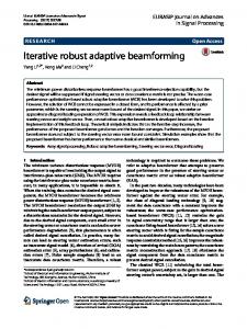
Adaptive systems imply a vast field o f research and development so the present discussion is restricted to the most common structures and algorithms. More involved discussions are available in the vast body o f literature, e.g. [1],[3],[31],[34], W ith only a negligible loss o f generality, the structure considered for the present purposes is that o f a linear combiner as sketched in Figure 1 below. It is always stable from the signal viewpoint, and, as mentioned in [3], can serve a variety o f applications from equalizers to neural networks to antenna arrays. The last application is o f primary interest herein.

Figure I: Linear combiner structure.

9


CHAPTER2

10

Essentially, the linear combiner serves to compute the inner product o f its complex coefficient N-vector W k with the signal-vector Yk to generate a scalar output signal yk as W? Y k . y k for the k-th iteration at time

r = fcAr .where

Ar

[J?] = T r{g {Y Y H)\ = Y h Y,

as

long

as

0 < p < 2/Tr[R]

where

the

quantity

's t'le >nPut signal power.

It has been suggested that a better version o f the LMS algorithm should use the current signals, because the conventional LMS algorithm introduces an extra delay by using the past signals [22-24]. This results in a normalized LMS (NLMS) algorithm, which may be derived alternatively as in [31]. Here it is derived from the continuous time LMS algorithm to show how various versions o f the FRQN algorithm can be obtained.

In continuous-time the extra delay in the LMS algorithm vanishes in the lim it as It is given by the differential equation

r - j- W f l = - * W

a(r)W (r) * g y ( t ) r - ( t ) = - g Y ( t ) e '( t )

(46)

a t .J

where T is the open-loop averaging time-constant and the gain is required to be g > 0 for stability. The LMS algorithm minimizes the mean square error on average, but at each instant its direction o f change o f the weight vector is that which reduces the instantaneous squared error. That is because it uses the instantaneous gradient o f the squared error (which is also the gradient o f the instantaneous squared error) to estimate the true gradient o f the performance surface. The algorithm itself performs averaging intrinsically by its recursive nature, and the fact that each incremental change in W advances it only a short way to the final solution.


23

CHAPTER 2

To obtain the normalized discrete-time LMS algorithm, equation (46) is first averaged with the usual assumptions o f ergodicity and independence o f W(t) from Y(t). resulting in

r — W{t) dt

= -gR W (t) +gS.

(47>

This is then transformed to the Laplace domain and written as sTW(s) = -gR W (s) + gS(s).

A t this point one o f a number o f s-to-z transformations (see Appendix A) may be applied to convert it into the z-domain, e. g. the bilinear transformation

(49)

or the backward-difference transformation

(50) Ar Choosing the latter with

A r being the Nyquist sampling interval and transforming back

into the now discrete-time domain produces ■:AWk = -gR W t + gS

where

(51)

t = T /A t is the normalized open-Ioop time-constant. Upon "deaveraging" and

assuming that the signals or data represented in R and S include the current data at time t = k A t . this becomes


CHAPTER 2

24

t A ^

= - g Y J ? W t + s Yt r l = - g Y t e l

(52)

which compares with (45). However, this is not a causal updating expression for W k because ek also contains W k. To obtain a useful updating algorithm for W k. one again makes use o f the matrix-inversion lemma (see Appendix E) to isolate it as (53) where

(54) This leads to the updating equation (which compares with (16))

(55) with the time-varying step-size parameter given by

(56) i Since W k is still being computed at this (k-th) iteration, the available output is given by

(57)

to avoid the problems pointed out in connection with the more conventional form o f the LMS algorithm. The indexing o f Y and y in the two algorithms is not identical. It can be shown that i f p in the conventional LMS algorithm is normalized by Tr|R ), the outputs o f both LMS and NLMS are identical except for that o f the latter occurring one iteration earlier. Normalization is merely a convenient way o f ensuring that (13) is

R e pro duce d w ith perm issio n o f the co p yrig h t ow ner. F urthe r rep rod uction prohibited w ith o u t perm ission.

CHAPTER 2

25

satisfied, so there is effectively only one normalized LMS algorithm (NLM S), contrary to implications o f [22-24], In this thesis, the NLMS form as derived from continuous time LMS w ill be utilized, since it most closely resembles the convention utilized in the FRQN algorithm, making comparisons easier.

Note that on average,

Pt is a step-size parameter normalized by the signal

power, thus satisfying (13). Consequently (56) gives unconditional stability since the gain is usually g > > 1. (One would also expect to preserve this kind o f stability by the nature o f this s-to-z transformation, as shown in Appendix A .) Note that (56) is naturally prevented from becoming infinite when the

signal power happens to be zero. (In

practice, finite noise power would prevent that.)

Also note that, although (55) minimizes the current error with the current weights according to (52), it does not actually use the current error in computing the current weights, as that is not causally possible. Instead, it uses the a-priori error, (as does RLS), which also automatically avoids the problem o f instantaneous following o f the reference as its speed is increased, according to (55).

The RLS algorithm also minimizes the present error using the a-priori error. One type o f comparison o f algorithms should involve NLMS optimized with respect to speed and misadjustment. The common step-size parameter for achieving this in the conventional LMS algorithm is

P

°

= — —

Tr[R]

■

It makes the excess mean square error equal to the minimum mean square error [31]. Reference [26] contains a derivation for the corresponding condition in the continuous time LMS algorithm from which it can be deduced that


CHAPTER 2

26

— - 7>[fl] = l T 2 where G = g and

(5S)

6 /2 = A is the Nyquist sampling interval. This corresponds to 1 = p = ------------------------------------------------------( 59 )

T

in (55). It leads to an average step-size parameter via (56) given by P = — ?— , 2Tr[R]

(60)

which is close to the one typically used in the conventional discrete-time LMS algorithm. Therefore the corresponding optimal open-loop gain in (54)-(56) should be T 7>[R] or with

t

(61)

determined as 4N from the requirements for Nyquist-rate sampling and

sufficient correlation time (to be discussed in chapter 3)

g

2.3 -

7>[R]

(62)

The FRQN Algorithm in Relation to Similarly-Motivated Approaches

A Review o f Recent Literature:

This algorithm owes its genesis to the work o f Dr. R. T. Compton, Jr. o f Ohio State University. He published in 1980 a modification for the analogue, continuous-time LMS algorithm implementation popular for adaptive arrays at the time, which cancelled most o f the dependence o f its time-consiants on the covariance-matrix eigenvalues [4|. He pointed out in his introduction, that it was not intended as a digital discrete-time


CHAPTER 2

27

computational algorithm, because other such algorithms which circumvented the problem o f eigenvalue-dependent convergence properties already existed. Presumably he had in mind block-wise matrix-inversion (with order-of-N 3 complexity), and recursive least squares (with order-of-N 2 complexity). Present research and development efforts are directed toward achieving order-of-N complexity.

With the original intent o f [4] in mind, the present author modified Compton’s analogue loops to more exactly cancel their eigenvalue dependence in the time-constants, and confirmed

its constant convergence properties by analysis and

hardware

experimentation [5], It has beer, successfully implemented in some products for m ilitary communications applications. These depended on its constant-convergence performance in that it served to protect digital radio links which could not tolerate lengthy jamming intervals without loss o f synchronization, or other links which also used fast frequencyhopping to evade jamming. The analogue implementation had the advantage o f relatively low complexity and real-time wideband performance. For some types o f algorithms, this is still the case today [ 10].

By applying the matrix-inversion lemma to the finite-difference counterpart o f the original second-order differential equation o f [5], a discrete-time version o f the algorithm was created. However, for stability reasons, the original block diagram now took on the form o f a non-computable discrete-time network. This meant that a digital hardware implementation would have to be o f a different topology than that o f the original continuous-time servo loops, in order to be causal.


CHAPTER 2

28

The basic version o f this (FRQN) algorithm is written as

^ ( T V , - 2 TV,., * TV,.,) + t , [ y / ♦ g Y J kB](W t - TV,.,) =

(fi3)

- ~ s Y t YtH Wt ♦ g Y kri

where k denotes the k-th iteration, g is a loop-gain factor; W is the N-vector o f complex weighs or adaptive coefficients. Y is the N-vector of complex input or data signals and t , and t , are time-constants normalized by the sampling interval

A r . the latter determining the

overall convergence time, and the former being much smaller. The scalar r represents a reference signal, or a main-channel signal as in the case o f a (generalized) sidelobe canceller. Gamma ( y ) is a diagonal augmentation term o f the input signal covariance matrix.

It was shown in [5] that the original analogue version o f this algorithm follows the Newton-Raphson method o f minimization o f the penalty-function. according to a firstorder analysis. It is preferable to the gradient-descent approximated by the LMS algorithm because the former always converges at a fixed and selectable overall rate, whereas the latter is exceedingly slow and jittery in many practical situations [ 11.

The FRQN algorithm can have several versions, and in fact differs from the original discrete-time version originally developed for simulation o f the analogue continuous-time implementation. That one also had two time-constants. but the smaller one was limited to be greater than about 8 N due to the requirement for Nyquist-ratc sampling combined with that o f sufficient averaging time for decorrelation o f N different signal vectors. With some modifications, the FRQN algorithm runs well with the smaller time-constant set to N and the larger one to about 4N, and achieves much greater suppression ratios than the original. Other versions can be derived by applying different


29

CHAPTER 2

s-to-z transformations to the Laplace-transform o f the averaged original differential equation in |5]. (Such an approach is also applicable to other continuous-time stochastic adaptive algorithms.)

By specific references to recent papers on similarly-motivated improvements o f LMS and RLS algorithms, the unique properties o f the FRQN algorithm w ill next be illustrated. First, the difference equation for the basic (not optimized) version o f the FRQN algorithm is rearranged in the form o f a programmable, recursive weight-update equation as

(64)

with

a0 = x 2 (x, + y ), b0 = g + z2g,

parameters

were

Since Yk Wk t and

chosen

= 2 x 2(x, * y / 2 ) and bl = g x 2 = bt - g .

as y = l / x 2, g -

The

x2 = 4N a n d x, = x 2/4 .

Yk Wk 2 ate scalars, it is clearly o f order N. Its derivation and

refinements are postponed until chapter 3.

The FRQN algorithm is numerically stable and works with arbitrary array geometries and coupling structures. Initial comparisons in the same scenarios with LMS (actually NLM S) showed dramatic improvements o f convergence rates and weight jitter in the ill-conditioned cases.


CHAPTER 2

30

Perhaps the best-known numerically stable FRLS type o f algorithm is that o f reference [ 6 ], but it is not applicable to adaptive arrays, because their data vectors do not possess the requisite shifting property. That is true even for perfectly regular array geometries such as uniformly spaced elements along a line without mutual coupling. The technique o f reference [7] is applied specifically to adaptive arrays but requires a specific (uniform, linear) array geometry. In addition, there are concerns that its initialization does not guarantee global convergence. It relies on infrequent updates o f a spatial pre filter or beamformer. which are o f order-of-N; complexity. A related reference | 8 | addresses the convergence problem, but still relies on the special array geometry. It also refers to Compton's work [4], citing that the convergence is still slow for the smallest eigenvalues. Mention is also made o f a fast adaptive-array algorithm operating on a cascade structure known as a Davies tree, but it also requires a specific array geometry (either uniform linear or circular with a phase-mode network) [9], That technique does not always converge to the optimal state, and the computation is o f order N; . Like other techniques relying on specific array geometries, the accuracy o f the interference cancellation is always compromised by

the inevitable phenomenon o f mutual

electromagnetic coupling among the array elements.

As mentioned earlier, reference [10] describes an analogue implementation o f a neural network adaptive-array algorithm. It is rather fast (10 degrees o f freedom adapt in 0.1 ns) and cites digital LMS implementations as being slow and suffering from signalcancellation (due to weight jitte r [1]). It is similar to [5] only in that the response time is determined solely by resistance-capacitance (RC) time-constants rather than by computational complexity (which is o f order N:). Being analogue, it does not benefit from the inherent precision and flexibility o f digital implementations as the FRQN algorithm does.


CHAPTER 2

31

A common approach to improving the convergence properties o f the LMS algorithm is to vary its step-size. as for example in references [11] and [19]. That can modify the steepest-descent path only in a scalar fashion, i.e. it cannot change its shape to effect a shorter, more direct path to the optimum state. Usually the step-size is varied from large values for fast initial convergence to small values for low steady-state misadjustment and negligible signal-cancellation. It cannot achieve the homogenization o f all modal time-constants as in Newton-type algorithms, which are regarded as the most "efficient" in this sense [ 1], because that requires a matrix operation on the gradient estimate. It is also not always clear when the adaptation is in the "in itia l” stages and when it is in more "steady" stages in an arbitrary dynamic scenario, i.e. it has little relevance to non-stationary scenarios (footnote 5 o f [3]), unlike the FRQN algorithm.

A somewhat more potent approach is to use a diagonal matrix in place o f a scalar step-size in an LMS algorithm, as for example in [15]-[18]. In [15] the authors use a fixed diagonal matrix to keep the computational complexity low. It is calculated from the known signal structure, in this case measured echo characteristics o f a conference room. Being diagonal and deterministic, this gradient transformation matrix also cannot achieve the homogenization o f the LMS modal time-constants. References [ 16]-[ 18] are concerned with a varying diagonal step-size matrix, which effectively performs an automatic gain control function on the components o f the estimated gradient. That gets around the problem o f distinguishing initial adaptation stages from later ones, but its authors acknowledge some o f the comments to the effect that it may not work with long filters [18]. In principle, it still cannot achieve a Newton-type o f convergence to the optimum because the step-size matrix is diagonal, whereas the ideal step-size matrix is the inverse o f the array covariance matrix (as in the RLS algorithm, effectively) which is rarely i f ever diagonal.


CHAPTER 2

32

Attempts at effecting non-diagonal step-size matrices in LMS algorithms sometimes follow the approach o f transforming the data vectors so the covariance matrix o f the transformed data would become more diagonal. That may be done by passive array feed networks or beamformers. but does not work in general, because the required transformation is data-dependent and the beamformer is constrained to be fixed. Some improvement may result from using power normalization o f the beamformer outputs as in [ 20 ], but that cannot generally be relied upon to eliminate the eigenvalue disparities. To quote from the abstract o f that reference: "Since the Karhunen-Loeve transform (KLT) is the ideal transform for this application.and since the K L T is defined in terms o f the statistics o f the input signal, it is certain that no fixed-parameter transform w ill deliver optimal learning characteristics for all input signals. However, the simulations suggest that, with a little trial and error, transforms can be found which give much improved performance in a given situation." [20]. The FRQN algorithm does not have such limitations.

Algorithms which inherently orthogonalize the data and thus effectively equalize all the modal convergence rates are studied in [ 21 ] in the context o f adaptive equalizers. Fast quasi-Newton and conjugate gradient algorithms are quoted as being profoundly affected by extremely small amounts o f noise, even to the point o f instability in the case o f the conjugate gradient method. The self-orthogonalizing algorithms studied in that paper all have a computational complexity o f order N: and are applied only to tappeddelay-line or FIR types o f input signals. The FRQN algorithm is insensitive to noise in the data and is computationally simpler.

Less accurate but computationally simpler approaches to self-orthogonalization are described in [22]-[24], Actually, reference [22] does not claim to perform selforthogonal ization, but rather to enhance the stability o f the LMS algorithm by using the


CHAPTER 2

33

current weights and data in the weight-update equations. Reference [23] shows how to perform the corresponding weight-vector computations without having to compute the vector entries one at a time while holding the others fixed. It is essentially the same idea as the "noncomputable loop” for the LMS algorithm and may also be derived by application o f the matrix-inversion lemma to that kind o f loop. That was done in the process o f developing the FRQN algorithm. In the case o f the LMS algorithm, it has a similar effect as division o f the step-size by the total input power, which accounts for the unconditional stability o f the resulting MLMS algorithm. However, it does nothing to reduce its eigenvalue disparity, and provides the same output as the conventional LMS algorithm, but one iteration earlier. The same idea is responsible for the unconditional stability o f the FRQN algorithm. However, the FRQN algorithm also employs other features to effectively achieve self-orthogonalization, i.e. by normalizing its step-size with a higher-rank operator than the scalar signal power. The approach o f [24] is to use reduced-rank estimates o f this operator as a way o f generalizing the power normalization idea. Typically the rank is 1 or 2. While that is clearly suboptimal, its author has some concern that the "implementation complexity might be high." The optimal operator is the inverse o f the (up-to-date estimate o f the) input covariance matrix, which is closely approximated in the FRQN algorithm without excessive complexity.

The FRQN algorithm is similar to a second-order LMS algorithm described in [26], in the sense that it is also a second-order algorithm with similar complexity. When the gain o f the second-order LMS algorithm is such that all its modes converge with decaying oscillations, their envelopes have the same time-constant which is independent o f the eigenvalues. The oscillation frequencies, however, are directly related to them, which may compromise its stability with real-life stochastic signal. (Subsequent investigations during the course o f this work showed it to be unstable in discrete-time simulations in most scenarios.) Reference [26] was mostly concerned with analyzing its


CHAPTER 2

34

misadjustment under averaging and independence assumptions, and found it to be about half that o f LMS without the oscillatory behaviour (strangely enough).

Other adaptive algorithms which approach the convergence properties o f RLS keep appearing in the literature e.g. [25], but they are generally similar in some respects to those already mentioned. Those in [25] have order-of-N; complexity. Others involve a variable step-size parameter and an algorithm for adjusting it. In [29] the LMS algorithm incorporates an embedded gradient algorithm to adjust the step-size parameter effectively in proportion to the square magnitude o f the gradient in the original LMS algorithm. It minimizes the change in the mean square error. While it reduces the steadystate excess mean square error below that achieved by the LMS algorithm, it really is no faster. Typically it starts with a large step-size and adapts quickly (mostly in a nonoptimal direction), then reduces its step-size and slows down near the end o f adaptation to minimize coefficient jitte r. A refinement o f it uses a separate step-size parameter for each gradient component, in effect a diagonal-matrix variable step-size parameter. By contrast, the FRQN algorithm adapts the actual step-size and direction optimally, toward the Newton path, by an amount proportional to the difference o f the coefficient step from the optimal Newtonian one. As w ill be seen in a geometric interpretation, this happens relatively early in the adaptation process and is an intrinsic property o f the whole algorithm. Thus the stability o f both the coefficient adaptation and coefficient-step adaptation is assured.

Reference [32] describes an algorithm which is applicable only to FIR timedomain filters, as it explicitly depends on their structure for its computational advantages over the RLS algorithm. Unlike the FRQN algorithm, it w ill not work for general adaptive arrays. Reference [33] discusses LMS-type algorithms with diagonal-matrix variable step-size parameters, but with sign-change driven algorithms for adjusting them.

R epro duce d w ith pe rm issio n o f th e co p yrig h t ow ner. F urthe r re p rod uction prohibited w ith o u t perm ission.

CHAPTER 2

35

It is not clear that speed is increased, because all the simulation results show the LMS algorithm using the smallest step-size parameter while the innovative ones are started with larger ones, which tend to the smallest LMS one at steady state. The simulation results show the variable step-size algorithms to be little more than twice as fast as the LMS algorithm and to possess the same steady-state errors.

No decrease in

misadjustment is shown either.

Rather than "Newtonizing" the LMS algorithm. [36] takes the approach o f simplifying the RLS algorithm by using only the diagonal entries o f the estimated inverse covariance matrix in equation (36). It is thus equivalent to what may be the optimal way o f controlling the step size o f each weight component in the LMS algorithm. Results in [36] show only small improvements in the learning curves. An improvement in array pattern convergence was shown only for what turns out to be a well-conditioned scenario where the LMS algorithm is known to do well.

2.4 Applications and Further Motivation

The FRQN algorithm is intended for time-critical digital applications, where its convergence time must be known to lie within designated bounds and preferably constant and short. Compton's original motivation was to improve the convergence properties o f the then-popular analogue LMS algorithm, because in his experience it had a disappointingly low dynamic range, in the following sense [4]: In a typical aircraft communications application, an LMS adaptive array frequently gives rise to a highly illconditioned array covariance matrix. The ratio o f its highest to lowest eigenvalues is in the order o f the signal- or jammer-to-noise ratio, and so is the ratio o f its modal timeconstants. System requirements dictate a maximum allowable response (overall convergence) time for tracking signals and interference, and also specify a modulation


36

CHAPTER 2

bandwidth which must be protected from jamming. Consequently the slowest modes must converge faster than the maximum allowed response time, yet at the same time the fastest modes must not converge faster than some multiple (say 5) o f the reciprocal modulation bandwidth . to prevent distorting the signals [4). In Compton's experience, these requirements are frequently impossible to meet with LMS adaptive arrays over the dynamic range o f signals encountered in practice. That is, either the slowest modes are too slow or the fastest ones are too fast, so one needs to reduce the dynamic range of their time-constants or to eliminate their dependence on the eigenvalues. This is equally true in more modern digital implementations.

Other applications o f the LMS algorithm also encounter this difficulty, hence the ongoing research efforts to devise algorithms which have a fixed, controlled convergence and low complexity, as evidenced by the numerous references. The main virtue o f the LMS algorithm is its order-of-N simplicity o f implementation. Recently, numerically stable fast recursive least squares (FRLS) algorithms with order-of-N complexity have been devised for adaptive FIR filters [ 6 . 12J. However, they rely upon the shift property o f the data signal-vector which gives the covariance matrix a highly regular structure. This is possible only in applications having the FIR filter data structure, which is not the case with adaptive arrays. Therefore, more specific applications o f the FRQN algorithm are in time-critical digital adaptive arrays.

For example, adaptive arrays o f this kind can be used to improve the spectrum efficiency,

hence increase the capacity of,

new digital

cellular mobile

radio

communications systems [13,14], These typically employ digital angle-modulation schemes and either T D M A (time-division, multiple-access) or C D M A (code-division, multiple-access) signalling formats which require synchronization, hence are time-critical. The "job” o f the adaptive array is to cancel interference from other cell-sites where the


37

CHAPTER 2

same frequencies are reused, and to perform diversity combining o f desired signals so as to minimize multipath fading. They would typically be installed at the base-stations as receiving antennas and employ reference signals for optimal adaptation. In reference [ 14-J Winters explains the dynamic range limitations o f an LMS adaptive array in such an application, where a secure spread-spcctrum reference signal is used. As a possible solution, he mentions an early form o f Compton’s work [4], Being a digital extension o f Compton’s work, the FRQN algorithm is directly applicable here. Another application also investigated by Winters recently is for the North-American digital cellular system IS-54 [13], where he found the LMS algorithm incapable o f tracking signals and interference

even

from

slowly-moving

vehicles.

To

quote

from

his

abstract,"Results...show that the LMS algorithm has large tracking loss for vehicle speeds above 20 mph. but the DM I (direct matrix inversion) algorithm can acquire and track the weights to combat desired-signal fading and suppress r .erference with close to ideal tracking performance at vehicle speeds o f up to 60 mph." [13]. Assuming, as Winters does, that the RLS algorithm has performance equivalent to that o f D M I, the FRQN algorithm is also directly applicable in such a scenario, and is expected to yield similar tracking improvements but with only order-of-N complexity.

One application that came to mind as being particularly suitable for the FRQN algorithm is the base-station antenna system o f a high-capacity mobile radio network. Due to the high capacity,

the volume o f signal-processing dictates a digital

implementation. The concept is discussed more fully in chapter 4 on reference signals; see Figure 27 in that chapter.

The basic idea is that, in a mobile-radio network such as the cellular telephone system, each mobile would transmit exactly the same message simultaneously on two carrier frequencies (e.g. narrowband FM channels). A t the base-station, an adaptive


CHAPTER 2

38

array and a fixed-pattern antenna would each receive one channel and convert both o f them synchronously to the same IF or to baseband. The signal from the fixed-pattern antenna would serve as the reference signal for the adaptive array which receives the same message on the other frequency o f the transmitted pair. A t each o f the frequencies in the pair, signals from other mobiles would also be received, but only the message transmitted simultaneously on both o f them would be correlated among them: the interfering signals would not correlate among the two channels when converted to baseband. It is a situation o f "forced” spectral self-coherence. There being a total of M (M -I)/2 possible unique pairs o f frequencies in a set o f M frequency-channels o f a cell, this scheme potentially allows (M -I)/2 times more users to share the same spectrum. The first frequency is used M -l times, the second M-2 times, and so on (see Table 7 in chapter 4). The adaptive array forms optimal beams on all mobiles, nulling out all co channel users (and other interference) but the intended one corresponding to the correlated message it sends on the other channel to the fixed-pattern antenna. The co channel interference present in the fixed-pattern antenna’s receivers (reference signals) contributes to the minimum mean squared error (mmse). However, only the excess mean squared error (emse) contributes to the output noise. It is shown in Appendix D that the FRQN algorithm has an emse about M times smaller than that o f the NLMS algorithm.

For transmitting, the weights o f the receiving array processors would be used to form orthogonal beams on the mobiles in a transmit band very close to the receive band. (A passive beamformer could be used with the array to make the weights less variable with frequency. Alternatively, transmit signals could be duplexed on the same frequencies in time.) This prompted the author to call the system "TR A AAP " (Transmit-Receive Adaptive Antenna Array Processor"). It is a form o f SDMA (Spatial-Division, MultipleAccess) scheme similar to that proposed by [37] for certain cyclostationary signals. TRAAAP has similar advantages in capacity (see chapter 4). It requires no special


CHAPTER 2

39

synchronization or signalling format such as in T D M A or C D M A for reference generation and no additional base-stations to increase capacity as in cell-splitting. Handsets would be inherently compatible with existing single-channel-per-user (AMPS) base-stations oy transmitting on one carrier by default. The FRQN algorithm offers the required low misadjustment and computational complexity, as well as fast adaptation and robustness desirable in a high-volume digital implementation.

In TRAAAP and applications such as proposed in [37], as well as GSM mobile radio networks [38], tracking ability o f the adaptive algorithm is not as important as is its ability to converge in a limited amount o f time and with small misadjustment. The FRQN algorithm was found to possess these attributes to a significantly greater extent than the LMS algorithm. Combined with its computational sim plicity, they further motivated its development and characterization in this thesis.


Chapter 3 Algorithm Development and Characterization: 3.1 Development o f the FRQN Algorithm and Possible Variants

In short, the FRQN algorithm evolved from Compton's algorithm |4| (see also equation (72)) by first introducing a diagonal augmentation term into the matrix coefficient o f W(t) resulting in the analogue continuous-time architecture o f [5]. The motivation for this was to complete the cancellation o f the dependence o f the closed-loop modal time-constants on the eigenvalues o f R. This was eventually transformed into discrete-time and rearranged. However, the severe effects o f insufficient averaging time relative to those in Compton's algorithm became apparent when the time-constants were reduced in attempts to speed it up.

Before presenting the derivation o f the present version o f the FRQN discrete-time algorithm, it is instructive to examine the effects o f insufficient averaging times in the original continuous-time versions [4], [5],

The effects o f insufficient averaging time may be shown with the help o f a modified ftnal-value theorem o f Laplace transforms, applied to the original continuous time versions o f the algorithm. The final-value theorem o f Laplace transforms states that Lim W(t) - Lim s W(s). ts- 0

(55 )

In the modified, so-called "late-value" theorem, one simply lets s be small in sW(s), thereby allowing some approximations, then divides out s and transforms back to W (t). Small s implies large t. A t large values o f t, some averaging has taken place

40

R e pro duce d w ith perm ission o f the cop yrig ht ow ner. F urthe r rep rod uction prohibited w ith o u t perm ission.

41

CHAPTER 3

intrinsically within the adaptive algorithm so the higher-frequency terms are written as averaged, with their usual independence from the (lower-frequency) state variables assumed. To see the effects o f insufficient averaging, one simply omits this intrinsic averaging in the approximated late-value algorithm expression.

Applying this to the original continuous-time algorithm corresponding to [5], i.e.

T l T2 ^ ~ W (t) +T2 - i /

4 w{t) *

0

dr

&

(66)

\ l + gY{t)YH(t) W(t) = (dg )Y (t)r-(t) o

with

6 = T2I(T2 + T ,) = 1 since

Tz z. 5 Tt , one employs the usual treatment o f

ensemble-averaging and diagonalizing before transforming to the Laplace domain, leading to r i T2 s2\ ( s'> * r 2 ^

where and

* S K jsv„(s) + 6 ^ - i

is the n-th eigenvalue o f R,

jv„(s) = (6 g )b n\Cs)

(67)

F(s) = 1 , and

(6 g ) s b n{s) ------------------------------------s r 2 ( l + g i „ ) + ( l + g X „) 6=1

(Go;

is assumed. The effect is seen to be the

disappearance o f the second-order time-derivative term in the corresponding time-domain equation (as if t , - 0

), which for "late" values o f t becomes


CHAPTER 3

42

r 2 [7 + 8Y(i) Y B(t) ] 4 W(t) = - [ / + s y ( t) y " ( r ) ]w ;f) + (g )y (r)r-(f)

dt

(69)

(This corresponds to the steady state in the geometric interpretation in the next section.) When the averaging is omitted, one can apply the matrix-inversion lemma (Appendix E)

| / + g y (r)y " (r)I ' 1 = /

Y(f) - " W—

y«(f)y(t) ~ i / g

(70)

to rearrange this so it becomes

(71) U + g Y H(t)Y (t))

Clearly, when dW (t)/dt = 0. this does not converge to the correct (Wiener) solution for W . In effect, the absence o f averaging incurs a severe misadjustment.

On the other hand, Compton’s algorithm without averaging can be written directly from his formulation in [4] as

[ / + 2/fccy(r) y H(r) ] — W(t) = -2kY (t) Y H(t) W(t) - 2 k Y (t)r'(t) dt where k corresponds to gain

(72)

g l( 2 T 2) , c is a separate time-constant. By the same

rearrangement procedure, this simplifies to

4 ^ 0 = -y (r )y " (r m r )p (r ) - y(r)r-(t)P(r) dt

(73)

with

R e pro duce d w ith pe rm issio n o f the co p yrig h t ow ner. F urthe r re p rod uction prohibited w ith o u t perm ission.

43

CHAPTER 3

(74)

This is effectively the normalized LMS algorithm (NLMS) which w ill converge as close to the optimal (Wiener) solution as the old LMS algorithm [23].

For sufficient averaging time to give reliable correlation estimates and thus to promote quasi-Newton convergence behaviour, Compton derives the criterion in [4] which restricts

Tl a 2 N /B , where B is the bandwidth occupied by the signals in the

N-dimensional complex (2N real) vector Y(t). Coupled with the need for Nyquist-rate sampling o f those signals in a fully digital (i.e. software) algorithm implementation whereby

2 B s 1 /A r

(see Appendix A), this leads to

or equivalently to

Ti — =t,j4 N At 1

.

(75)

However, as Compton points out in [4], smaller averaging times may suffice to correctly estimate the rank o f R, suggesting that the degeneration to an LMS algorithm with decreasing T, may be rather "graceful” .

Realizing that the original loop type o f architecture was no longer a constraint in a digital computational implementation, the diagonal augmentation terms were dropped from both the W(t) and dW(t)/dt matrix coefficients in the next version. The idea was to maintain exact cancellation o f the eigenvalue dependence o f convergence times while


CHAPTER 3

44

allowing the algorithm to converge to the correct (Wiener) solution even with shorter averaging times. In most respects it did this, although the condition (75) was still necessary. Its weights (state variables) also tended to acquire damped oscillations and to wander in ill-conditioned scenarios, although the output residue was not appreciably affected. Stability analysis showed that the gain "g" had to be sufficiently large so that g \ m > 4 7 ,/7 ",

to prevent oscillations and to assure a fixed dominant time-constant

for convergence speed.

Consequently, an augmentation term o f

y = 1 /r, 1 was added to the matrix

coefficient o f dW/dt to overwhelm the minimum-eigenvalue term, thus creating the basic version o f the FRQN algorithm, equation (63). If transformed back into continuous-time and its parameters suitably adjusted, it corresponds closely to Compton's algorithm with a single-pole averaging filter. It converges to the correct solution without wandering or oscillating, and allows for reduction in averaging times without completely degenerating to the NLMS algorithm. It benefits from the "persistent excitation" property because o f the absence o f only one leakage term. That term makes the integrator which outputs W(t) "leaky” , which effectively depletes its memory about the dimensions o f the sampled signal-vectors, so it needs longer averaging times as in equation (69).

One can generalize the basic version o f the FRQN algorithm by using various sto-z transformations to create corresponding discrete-time versions o f Compton's algorithm, and by adjusting their parameters (gains and time-constants). Similarly, one can also do this to the LMS algorithm, to e. g. minimize its misadjustment while not reducing drastically its convergence speed.


45

CHAPTER 3

By following the procedure used to transform the differential equation for the continuous-time LMS algorithm (46) into discrete-time (55),(56), the differential equation for the original algorithm (66) is similarly transformed into discrete-time. (Alternative s-to-z transformations are also possible, giving rise to other version o f the FRQN algorithm, as shown in Appendix C.) Equation (63) is obtained when only the derivativeweights’ coefficient augmentation term is retained as described above, corresponding to the continuous-time version

i

\

Tl T2^ W { t ) + T1[ y I + g Y{t)YH( t ) \ ± W { t ) + g Y ( ! ) Y H( f ) W ( t ) = g Y(t)r-{t) \ d r at \

ii_________________________________________________________________________________________________________________ ii

The procedure to obtain equation (64) involves a straight-forward but tedious application o f the matrix-inversion lemma after all the Wk terms have been isolated on the left-hand side in equation (63):

[ ( t 1TI + . 2Y) / ^ ( i + x2)y l ytf f ] ^ + [ - 2 x 2( t 1+ Y/ 2 ) / - g T2r i r / ,] ^ . 1+ (76) + TI TSWt - 2 = « 1W Let

a0 = x ,( x , + Y), b0 = g ( l + x ; ), a, = 2 x ; ( x I + Y/2 ), b, = g x 2, and write

Using the matrix-inversion lemma to isolate W t on the left side, the above equation becomes


CHAPTER 3

46

y j

‘o

:

° o lh + Y?Yt

T,T

I-

a,'o

v * w

" K

, (78)

Yk Ykh

Yt Yk

% lb 0 - Y ? Y k

V*>o 2 x 105 iterations overnight on an IBM-compatible,

-386/33MHz personal computer, using the A T -M A T L A B 3.5k software for modelling. No signs o f instability or error-accumulation were noticed: the residual error remained constant in stationary scenarios.

Both algorithms were next tested in "optimal", fully-adaptive arrays using reference

signals.

State-variable

and

output

error

evolutions

were

compared

quantitatively. These results are discussed in the next section.


60

CHAPTER 3

3.4 Quantitative Simulation Comparisons o f Basic FRQN and NLMS Algorithms:

The FRQN and the NLMS algorithms were simulated in a more realistic, mobileradio environment. A perfect replica o f the desired signal was assumed to be available to use as the reference signal. The algorithms were configured to minimize the mean square error using 4 directive elements spaced half-wavelength apart along a line. One source o f desired and three independent sources o f interference signals within 3 dB of the desired-signal level were modelled as 25 kHz band-limited noise at 850 MHz carrier frequency. A ll sources were capable o f motion, but fading and shadowing effects were not modelled. Only 2-ray elevation multipath propagation was modelled, with slightly randomized specular reflections from the ground for each signal, but no delay spread. The signals were modelled as independent complex Gaussian pseudo-random sequences bandlimited by phaseless filters to about 25 kHz, sampled at 60 kHz. They represented the received signals at baseband. Independent random noise corresponding to a noisefigure o f 10 dB was injected into each o f the 4 receiving channels, resulting in SNR of about 63 dB for the desired signal. (Note that "noise" does not include "interference".)

The adaptive-array antenna was assumed to be mounted on a mobile-radio basestation mast 50 m above a near-perfectly conducting infinite plane earth, and consisted of N = 4

elements spaced at 18 cm intervals along the

directive in the

90°

0°

radial. Each element was

radial direction and connected to one coherent receiver and

complex weight. An attempt was made to normalize the residual error to unity (0 dB) when the weights were in their initial zero states.


61

CHAPTER 3

Similar scenarios as in the preceding section with the sidelobe-canceller configuration, were tested with these error-minimizing configurations o f the algorithms. Antenna patterns were not plotted this time, since in general the sources could be at different elevation angles, requiring a laborious 3-dimensiona! illustration o f the spatial nulls formed on them. The relative performances o f the two algorithms were similar as before. When the simulations were repeated without noise and motion, no noticeable differences were observed upon introduction o f source motions.

Briefly, the two scenarios consisted o f 4 independent mobile signal sources 2 m above ground and 3 km radially distant from the basestation. In the "orthogonal" (wellconditioned) scenario the sources’ bearings relative to the line o f the array were 90°, 140°, 52°, 32° -Their corresponding transmitter powers were 47, 44, 43 and 50 dBm and velocities were 60 km/hr@ 180°, 30 km /hr® 180°, 130 h n /h r @ 0°, Okm/hr, respectively. In the "parallel" (ill-conditioned) scenario, only the interferers’ bearings were changed, to

72°, 71°, 70°,

in the same order. The desired signal remained at

90° , directly in front o f the array.

Convergence performance and relevant algorithm parameters are more tidily summarized in Tables 2(a), 2(b) and 3 and the Figures which follow . The last table shows a variation o f the FRQN algorithm in which the time-constants were reduced in an attempt to speed it up. In fact, the resulting effect was more the opposite, due to reduction o f the averaging time and consequently more NLM S-like convergence behaviour. This illustrates that a trade-off exists between averaging times and convergence times o f the FRQN algorithm.


CHAPTER 3

62

To help interpret the following results, the theoretical values o f the NLMS closedloop time-constants were calculated according to Appendix B as

T»=T/(S1»)

(86)

and theoretical convergence times were given approximately by * = 5 t n num.

(87)

In the orthogonal (relatively well-conditioned) scenario the NLMS weights converge in the theoretically expected 250 or so iterations (the squared error in k=500). The FRQN algorithm takes longer than the expected averaging time in selecting

r,

and

5 t, t;

iterations because there is some loss o f smaller than advised by equation (75).

Increasing these time-constants eventually causes it to converge in the theoretical number o f iterations; unfortunately that is more than NLMS takes in this scenario. The current values o f these time-constants represent an empirical near-optimal compromise between faster, more LMS-like (variable) and slower but more constant convergence rates for the FRQN algorithm.

In the ill-conditioned scenario, this selection o f time-constants is seen to result in only a moderate increase in convergence time compared to that o f the NLM S algorithm. The NLMS algorithm converges practically in 5 times the second-slowest time-constant, as the slowest time-constant governs a mode responsible for only a negligible portion o f the output error power.


CHAPTER 3

Table 2(a):

63

Well-Conditioned Scenario, llcnuons to

Algorithm

converge, k

5.8 x 10'°

Opcn-loop

Closed-loop

Figures:

time-

time-

w eights (a)

constants

constants

e rro r

T, = 16

it

300

. N = 4.

V*

FRQN

O pcn-loop gain, g

= 28.05.

(b)

7(a) 7(b)

x ^ l. 8 7 NLMS

500

1.71 x 1010

8(a)

r - 16 xi = 2.99 xc = 53.7

8(b) x ^ S .9 6

Table 2(b): Ill-Conditioned Scenario, Iterations to

Algorithm

FRQN

Open-loop gain, g

converge, k

1000

4.9 x 1015

^n ul!

^"min

6,54

x

106.

N = 4.

Open-loop

Closed-loop

Figures:

time-

time-

w eights (a)

constants

constants

e rro r

X,

=4

x; = 16

(b)

9(a) 9(b)

^ = 1-26 NLMS

15000

9.33 x 109

10(a)

T = 16 t a =4.86

2.8 x10s 10(b) 8.3 x lO 6


CHAPTER 3

64 Proposed olgorithm weights vs. k

fterotion number. k

Figure 7(a): Weights o f FRQN algorithm in well-conditioned scenario.

Convergence of "DALG03.M"

L o g d O o f ite r o tic n o r s c m p le n u m b e r k

Figure 7(b): Squared output error o f FRQN algorithm in well-conditioned scenario

R epro duce d w ith perm issio n o f the c o p yrig h t ow ner. F urthe r rep rod uction prohibited w ith o u t perm ission.

65

CHAPTER 3

NLMS Mights vs. k

Iteration number, k

Figure 8 (a) Weights o f NLMS algorithm in well-conditioned scenario.

Convergence of "DlMS.M"

Loq©10 o f iteration o r sample num ber k

Figure 8 (b) Squared output error o f NLMS algorithm in well-conditioned scenario


CHAPTER 3

66

Proposed olgorithm weights vs. k

‘5 *

_e>

a v

10®

101

102

105

Keroticn number, k

Figure 9 (a) Weights o f FRQN algorithm in ill-conditioned scenario

Convergence of "DALG03 .M"

10® I----------- 1------ 1----, 1 I I I | |----------- 1------ 1---- ! r I I H-

1 0 “ * * -------------- 5--------

10°

■ ,

I I i ■ i-------------- i-----1— i

101

.....................

102

1--------.

■ ■

105

LogOIQ o f iterot'on o r sample num ber k

Figure 9 (b) Squared output error o f FRQN algorithm in ill-conditioned scenario


67

CHAPTER 3

NLMS weights vs. k

5

A 3

2

0

Iteration number, k

Figure 10 (a) Weights o f NLMS algorithm in ill-conditioned scenario

L o g d O o f iteration or somple num ber k

Figure 10 (b) Squared output error o f NLMS algorithm in ill-conditioned scenario


CHAPTER 3

6S

The Table below and subsequent Figures illustrate that simple reduction o f timeconstants must be traded o ff against degeneration to more NLMS-like convergence behaviour. While it results in faster convergence in well-conditioned scenarios, convergence in ill-conditioned scenarios is slower, as is the case for NLMS. The same adaptive array system and scenarios were used as in Table 2(a) and Table 2(b). but the time-constants o f the FRQN algorithm

were reduced to

x, = 3N = 12,

and

x, = t , / 5 =2.4 .

Table 3: Basic FRQN Algorithm With Reduced Time-Constants. Scenario

Iterations to

X;

Converge, k

WellConditioned

Figures: Weights (a) Error (b)

11 (a) 200

2.4

12 11 (b)

IllConditioned

12 (a) 2000

2.4

12 12 (b)

R epro duce d w ith perm issio n o f th e c o p yrig h t ow ner. F urthe r rep rod uction prohibited w ith o u t perm ission.

69

CHAPTER 3

weights vs. k

Iteration number, k

Figure 11 (a): Weights o f FRQN o f Table 3 in well-conditioned scenario.

L o g d C o f iteration o r somole num ber k

Figure 11 (b): Squared output error o f FRQN algorithm o f Table 3 in wellconditioned scenario.


CHAPTER 3

70

Proposed algorithm weights vs. k

Iteration number, k

Figure 12 (a): Weights o f FRQN o f Table 3 in ill-conditioned scenario.

Convergence of "DALG03.M"

10-3

L o g d O o f iteration o r sample num ber k

Figure 12 (b): Squared output error o f FRQN algorithm o f Table 3 in illconditioned scenario.


71

CHAPTER 3

3.5 Refinements of the Algorithms:

Some refinements o f the NLMS and FRQN algorithms become useful in their discrete-time forms. Specifically, it is legitimate to allow

g- ~

in both algorithms

without fear o f instability, unlike in their continuous-time counterparts. Furthermore, because the available outputs always use the weights o f the previous iteration, there is no danger o f producing a useless output signal stripped o f information.

The lim iting form o f the NLMS algorithm as (i-o o

g - » is obtained by letting

in equation (56) and substituting it into equation (55). This lim iting form has

eliminated the open-loop gain and time-constant as parameters from the NLMS algorithm, thus simplifying it as well as speeding it up to its maximum speed [35]. Slock has a different explanation for "instantaneous" adaptation based on a projection interpretation o f NLMS as g - oo in [35]. The refined form o f the NLMS algorithm is therefore given by equation (55)

(88) j.:» v.-un pt = l / ( y / , y l) , driven effectively by a t according to

(89)

and its available output is still as in (57)

yt ~ w " { Y k .

Although now the closed-loop

time-constants cannot be determined by analogy with the continuous-time form as in equation (86)with finite g, the discussion following equation (56) to (62) and in Appendix B serve to show that convergence times w ill be halved by this refinement, as was indeed observed in simulations.


CHAPTER 3

72

A corresponding form approach, i.e. letting setting a0lb 0 = 0

o f the FRQN algorithm can be obtained by a similar

g - ~ in its recursive update equation. It has

the effect of

in equation (80). When the simulations in Figures 7 and 9 were

repeated with this algorithm,

nochanges in performance were observed. It was also

verified to be numerically stable in long runs, as well as in theory (in the averaged sense), for stationary scenarios.

Another refinement o f the FRQN algorithm was motivated by resorting to its continuous-time original form. Looking at equation (69), it may occur to one that if g on the LHS was reduced, then the closed-loop time-constant would also be reduced by the same amount, say q. Carrying this idea into the discrete-time form has the effect of changing the parameters (in equation (76) for example) to

(90> It was found by simulation that if the equivalent o f the entire LHS was reduced by q, excessive ringing o f the coefficients would occur. The value o f q = 2 was found to be nearly optimal: higher values tended to increase ringing and convergence times, since the diagonal term on the LHS then became effectively larger, resulting in loss o f QN behaviour. (As

q - «> with

y =l

, the FRQN algorithm becomes an "ordinary"

second-order LMS algorithm which behaves essentially like the LMS algorithm except for possible ringing oscillations o f various frequencies in the coefficients. A version of it is analyzed in [26].) Although the geometric interpretation with q > 1 now suggested that the weight steps would converge toward the Newtonian direction more slowly, since equation (83) would become

v ^ P )]

(91)


73

CHAPTER 3

the steps in that direction would be q times larger. Besides, the infinite g would ensure that division o f the RHS by q would not pose a serious threat to the time-constant o f adaptation o f the weight steps. The complete refined FRQN algorithm is therefore given by

(92)

wilh a0 = t 2( t , + y ),

= 2 t , ( t , + y /2 ), y = 1 /x ,, q =2, t , = 4 N , t , = t 2/4, and oulput

by

(93)

It ran with the predicted two-fold increase in speed for > 105 iterations without signs o f divergence. The following simulations illustrate its superior behaviour with respect to that o f the refined NLMS algorithm. Theoretical mean squared error (mse) and minimum mean squared error (mmse) are plotted for both algorithms in stationary scenarios. They are derived in detail in Appendix D. Results o f simulating the same scenarios with the RLS algorithm are also included. It was refined only in the sense o f choosing version II RLS from [31, pp. 484-485] with the time-constant o f FRQN used to determine the forgetting factor as A. = 1 - 1/ t , It was initialized with

, since both parameters affect the tracking behaviour.

= / / (0.001

y"

} /N ) , in keeping with [31],


CHAPTER 3

74

The scenarios in Figures 13(a) and 13(b) to 18(a) and 18(b) are the same ones as in Figure 7 - 1 0 but the signal sources are totally stationary. (These scenarios were set up to reveal algorithm behaviours near both extremes o f scenario conditions and have been useful in early detection o f instabilities and excessive residual errors in algorithm variants. Simulation o f fast fading is deferred to later sections where the NLMS. FRQN and RLS algorithms w ill be compared in adapting with binary desired signals whose biterror-rates (BER) w ill be computed.) As mentioned earlier, the parameters in Tables 2(a) and 2 (b) remain the same in the following simulations except for g being infinite, the closed-Ioop NLMS time-constants being effectively halved, and q = 2 halving those o f FRQN as well.

The bumps in the approximate theoretical mse curves for the FRQN algorithm are believed

to

be

harmless

artefacts

V * 2) *‘ &{Wt - l Wi_l + Wk_2Wt'_1)l2

caused

by

the

approxim ation

which was used in deriving them. They

disappear as k -» CO .


75

CHAPTER 3

Convergence o f FRQN in the m ecn (orthogcnci,stationery)

6

5

A 3

2

1 0

Iteration number, k

Figure 13(a): Weights o f FRQN algorithm in well-conditioned scenario.

Convergence o f FRQN in the mean scucre (ortogonol, stationary)

10-' ':A -jjrio ri squared; error of single run

i :!?' Acpraxrnqte theoretical m$e

•Minimum.jneoa-'-ectwre^-fgroc-

IIP LogOlO o f iterotion o r sample number k

Figure 13(b): Squared errors o f FRQN in well-conditioned scenario.


CHAPTER 3

76

Convergence cf NLMS In the mecn (orthogcnol,stationery)

c*

'5 *

A Yiivr*.

iteration number, k

Figure 14(a): Weights o f NLMS algorithm in well-conditioned scenario.

Convergence o f NLMS in the meon souore (orthogonol.etolionory) 10°

; A -p r|c rt aquored error of fcingle Kin

•^inrryrurrr'meon-tquoTnj1

2 103 LogOlO of Iteration o r eomple num ber k

Figure 14(b): Squared errors o f NLMS in well-conditioned scenario.


TJ

CHAPTER 3

Convergence of RLS in the mecn (orthcgoncl, stationery)

0 ik

10 ®

Iteration number, k

Figure 15(a): Weights o f RLS algorithm in well-conditioned scenario.

10° 10-’

Convergence o f RLS in the meon acjuore (orttiogonci. atctionory)

A-pirlert scucrefl error o f single!

riiii I

■o 10-J u* & 10-3 t 10-* 0 73 10-= 1 10*« ...Ukumbm.»eon--BiqU04«d«eRcoi

4 10-7

10’

102

lo g © 1 0 o f iteration or ecmple num ber k

Figure 15(b): Squared errors o f RLS in well-conditioned scenario.


CHAPTER 3

78

Convergence o f FRQN in the mean (parallel, stationary)

Marction number, k

Figure 16(a): Weights o r FRQN algorithm in ill-conditioned scenario.

Convergence of FRQN in the meon sguore (porollel, etationory) ■jprloH Itjiic re d error of single njn 1 0 -1

‘Wfnirr'um'moon 3 ^

10-r‘— 10®

LogOtO o f iteration o r sample num ber k

Figure 16(b): Squared errors o f FRQN in ill-conditioned scenario.


79

CHAPTER 3

Convergence o f NLMS in the meon (poralW , etct'oncry)

. '

»j’ kiiu*[f?] =T.Xn ■The other quantities are the same as those for the NLMS learning curve in a stationary environment. In steady state the FRQN excess mean squared error was found to be given by


CHAPTER 3

88

mmse

emse «

(106)

with 4 P~g

2 p T : (2pT1

* 2 p zzlq ) Y HY

serving a role similar to that o f p in the NLMS algorithm. It was assumed that in p. Y " Y = T r | R] , An optimal value o f p which minimizes emse was sought within the limits 0< p < 1

in Appendix D. but was found not to exist. As g -

o f the NLMS algorithm with with

p k n< 2 and

p Xn-e2

. the misadjustment

is emse/mmse = 1. Under similar conditions

p =1 / 2 . the FRQN algorithm already has a much smaller

misadjustment than NLMS. given by

(The value o f

p =l

emse

1

mmse

1 + 2 x,/q

, < 1

(107)

creates an explicit potential condition for divergence and w ill not

be used.) Figures 20 and 21 confirm that, for the same convergence speeds, the FRQN algorithm (92) has a much smaller misadjustment in steady state than the NLMS algorithm ( 88 ). as predicted by (107) above.

Convergence in the mean square in a non-stationary environment was also analyzed, specifically for tracking error with the performance-surface jittering in position but not in shape. Its random movement was again characterized by a first-order Markov process modelling the optimal coefficients, which jittered much more slowly than the adapting coefficients (quasi-stationary assumption). For the FRQN algorithm with


CHAPTER 3 p = 1 /2

89

the mean squared tracking error in the quasi-steady state was tbund in

Appendix D to be approximately given by

tmse

1-J L

-

9(1 +

(101

1 -J L

-

1

where

o\

- -

*

!

2

-

1-

is the variance o f the optimal weights and

stationarity. The dependence on x 1, t ,

is their parameter o f non-

is negligible and 4> is slightly less than 1 and

P = 9 / ( ( 9 + T2) 7 r [ / i ] )

Since

t , / ^ > 1 the FRQN tracking error would be greater than that o f NLMS.

Indeed simulation results near the end o f this section show that the FRQN tracking error grows faster than that o f NLMS as the source velocity o f the desired signal (hence also its fade rate or Doppler) since $ and

increases. That corresponds to decreasing , but

ate not easily quantifiable from the scenario parameters, the

contribution o f the tracking error may not dominate the total mse in (96).

Some further refinements with respect to improving tracking performance in nonstationary environments were also conceived. They do not affect the foregoing expressions for mean squared errors, because the same approximations still hold. To illustrate, it is instructive to consider the instantaneous updating equations in terms o f projections parallel to (onto) and orthogonal to the subspace spanned by the data or input


CHAPTER 3

90

vectors Yk. (Similar reasoning in [39] inspired this approach.) For example, the NLMS algorithm ( 88 ) or (89) can be rewritten as

(109)

where the projection orthogonal to the current data Yk is recognized as

( 110)

and its complementary projection onto the current data subspace is simply

( 111) Note that

( 112) so that (109) can be rewritten as

(113) The bracketed expressions in (113) effectively represent the nulling components o f the weight vectors. When those are orthogonal to the current data,

Py has no effect on

them so they are not updated in (113)5. That is the correct behaviour . because being orthogonal to the data means that they are doing their nulling job, as their inner product with Yk is zero.

? Since alt the past and present data vectors Yk are not m utually o rth o g o n a l, the o rd e r o f the projections affects die outcom e 134). It is im plicitly assum ed herein that in a stationary steady state, the history o f projections relative to the data v ectors has had the sam e effect as using the orthogonal basis vectors which span the data subspace, in place o f the data vectors them selves.


CHAPTER 3

91

Supposing that this happy state has existed in a stationary scenario, the NLMS algorithm having converged, whereupon the current data suddenly sprouts a component which is not orthogonal to the nulling components o f the weights, i.e. falls within the subspace spanned by

t ) . Then (H^ , - S, k)

w ill no longer equal the LHS

o f (113) and the LHS w ill be updated to equal the new RHS. because the new Py affect w ill

( B ’j . j - Sj k) begin

tracking

w ill

with the change in the data. That is to say. the NLMS algorithm this

non-stationarity

in

the

data.

(As

an

aside,

note

that Yk Wt = r'k according to (109). but it is not an available output at iteration time k.) Therefore the "gain" in the NLMS algorithm may remain infinite as in ( 88 ) and (89).

Now consider the FRQN algorithm. It is instructive to examine it in terms o f the geometric interpretation, but on an instantaneous basis. To that end. equation (91) is rewritten in the form o f (82) as

-1 = -

T,

Recall that

(114)

I *g - ) y j ? U )

(et |2 = Yke'k , which is parallel to the current data vector Yk . It was

desirable to make g - ~ so as to promote Quasi-Newton (QN) convergence in the stationary case. The implications o f that in (114) would be to effectively neglect the diagonal augmentation "I" in the middle term. i.e.

T , A ( t 2A w t ) = ^ £ [ ^ ( ^ a b ^ - s v ;

a *•

J

.

( i i s>

Now the middle term is always parallel to the last term in (115). That is because < .-glq)[Y kYkHU-:2M Vk_1) = ( - g lq ) ( Y kHYt )P'Yi(-:1AWk_l ) ,

i.e.

it

is

directly

proportional to a projection o f A Wt _t onto the subspace spanned by the current data vector Yk . and

-g Y ke ’t

is simply a scalar multiple o f the same data vector.


92

CHAPTER 3

Supposing now that the happy state exists whereby the scenario is stationary and the weight steps move along the QN optimal direction toward

W

i.e . A 2

= Q on

the LHS o f (114) and (115). If the data suddenly becomes non-stationary. but this time in such a way that it sprouts a new dimension which is orthogonal to ( t : A l f w ) in particular,

t hen

that

w ill

because / " ( t . A K ^ ) = ( / " -

produce

no

c h an ge

A IT ,.,) .where

in

AW ^) =0

(115) Thus

the scalar coefficients o f the augmented data vector in both terms on the LHS o f (115) remain the same, consequently no change in the weight steps' direction w ill occur in the RHS o f (115) either. The weights may be adapting, but not tracking the change in the QN direction brought about by the data non-stationarity. However, a change w ill be produced in (114) with finite g, because the weight step is not entirely projected onto the data subspace. Therefore a finite "gain" g is required to maintain near-optimal QN tracking whereby the weight steps are always redirected toward the optimal direction leading to W

in all types o f non-stationary scenarios. To remain sufficiently close to

QN behaviour in ill-conditioned scenarios, it is desirable to keep

(116)

according to (114). so the optimal FRQN algorithm for non-stationary scenarios would be given by equation (80) with (116). i.e.

w* = 'T 1 *

(80)


CHAPTER 3

with

a0 =

+ y ) , *0

* ':/