FAST SCREEN MAP LABELING – DATA-STRUCTURES AND ALGORITHMS Ingo Petzold, Gerhard Gröger, Lutz Plümer Institute of Cartography and Geoinformation, University of Bonn, Germany, http://www.ikg.uni-bonn.de e-mail:
[email protected],
[email protected],
[email protected]
ABSTRACT This paper presents a new and very efficient technique for automatic labeling of dynamically generated screen maps. Such screen maps are frequently created in the course of the interactive navigation in a geographic information system. Since screen maps have to support the functions zooming and scrolling, the label placement must be achieved very fast. Therefore we developed a concept which separates the labeling process into two phases. Calculations are shifted in a socalled preprocessing-phase as far as possible. Thus, the number of time consuming operations in the time critical interaction-phase is reduced and the operation zooming and scrolling can be realized very fast. Our concept supports labeling of point objects as well as labeling of line and area objects. The separation in the two phases is achieved by a new reactive data-structure which is called reactive conflict graph. In the preprocessing phase, it stores information about all potential conflicts. During the interaction-phase this structure is optimally exploited and leads to a labeling in an efficient and a cartographic adequate way. 1. INTRODUCTION These days screen maps are the essential part for visualization of customized maps, and for interaction with geographical information systems (GIS). Text is essential for orientation and information. Imhof has formulated cartographic rules for map labeling (1), which may well serve as a base for automatic procedures aimed at readable maps with good orientation and information density. In contrast to static (paper) maps, the resolution of dynamic (screen) maps is much lower, and the size of screen maps, is restricted by the screen size. Thus screen maps are shortlived and must be generated on the stroke-of-a-key. Additionally, the labeling systems must support scrolling (changing the map clipping), zooming (free choice of scale), and integrating layers of different thematic themes in real-time. a)
Essen
Bochum
Dortmund Hagen
Düsseldorf
b)
Essen Düsseldorf
Wuppertal
Wuppertal
Bonn Bad Godesberg
Hagen
Leverkusen
Leverkusen
Köln
Bochum Dortmund
Köln
Bonn Bad Godesberg
Figure 1. Scrolling (changing the map clipping) leads to a movement of label positions. Scrolling of a map causes new labeling (see Figure 1). Also zooming a map not only requires changing the scale but also modification of the label size. A higher scale provides more details and larger labels. Thus zooming is not just a simple blow up or scale down of a map like a photo. Label placement for ordinary static maps is already pretty complex. If, in addition to the normal constraints, zooming and scrolling have to be supported and very short response times have to be achieved, complexity is increased considerably. From a computer science perspective the labeling problem is also very complex (2). This paper provides a general approach to handle this additional complexity. In order to avoid the conflicting demands between quality and running time, our approach is to divide the labeling process into two phases: a preprocessing-phase and an interactionphase. In the non-time-critical preprocessing-phase a so-called reactive conflict graph is constructed. This graph stores potential conflicts and necessary labeling information depending on the scale of occurrences. In the time critical interaction-phase efficient algorithms extract matching information and yield a preselection of the objects to be labeled in the desired scale. Our concept incorporates labeling of point objects as well as labeling of line and area objects. The reactive conflict graph integrates all those object types homogenously and scale independently. A major improvement to previous approaches is that the labeling is not restricted to discrete positions. Instead we use sliding labels in labeling space, which satisfies cartographic principles.
I. Petzold, G. Gröger and L. Plümer: Fast Screen Map Labeling – Data-Structures and Algorithms
1/10
A frequently used operation in GIS is the combination of several different thematic layers. The existing conflict-free labeling for each layer must be merged into a joint labeling. To retrieve the joint labeling, we developed a method to merge and exploit the layers’ conflict graphs into a new general one during the interaction-phase. This paper is organized as follow. The following section gives a short introduction into the basics of labeling screen maps. Afterwards the concept of the reactive conflict graph is separately presented for the preprocessing and interaction-phase. The paper concludes with a compilation of labeling approaches and our conclusions. 2. LABELING OF SCREEN MAPS This section introduces in some foundations of map labeling and techniques which will be used in the presented approach. At first we will discuss the subtle differences between traditional paper maps, also known as static maps, and screen maps, also known as dynamic maps. On the one hand, screen maps should have the same high (labeling) quality as paper maps and on the other hand, there are several technical restrictions and guidelines. Both the size of a display and its resolution, at one and the same time, is a fraction of the size and resolution of paper maps. This leads to less map objects and to a less filigree representation of them. The smaller map clip and additional demands for screen maps leads to the screen map functions scrolling (changing the map clipping), zooming (free choice of scale) and integrating layers of different thematic layers. As a result of the restrictions and the described functions, screen maps are short-lived. For a user-friendly interaction these maps must be generated on the stroke-of-a-key. Due to the reduced number of map objects and objects to be labeled, the labeling process is eased compared to paper maps but still most complex and time-consuming as shown in section 5. 2.1 Approximation of Labels Instead of working with the complex geometric shapes of labels to be placed, the algorithms use approximations. Figure 2 shows different kinds of possible approximations. To reduce the running time the simple approximation by a rectangle (Figure 2 b)) is used in our approach. a)
b)
Labeling
c)
Labeling
Labeling
d)
Labeling
Figure 2 A label, shown in a), and its possible approximations by label boxes (b) to d)). For easy handling and fast geometric calculations the approximation by a simple rectangle will be used in this approach b). 2.2 Label size in dependency of the scale In connection to screen maps and its zooming function, the question of dependency between label size and scale arises. The size of the label is not growing or shrinking in proportion to the map scale, which causes the relabeling after each zooming/change of scale. The label size (label) could be approximated by an exponential function for a destination scale (scale) in dependence on a reference size (labelrefScale) and reference scale (refScale) as follows: scale labelscale = labelrefScale refScale
value
with value ∈ [0.07..0.15] the growing and shrinking can be adjusted. More details can
be found in a previous paper (3). 2.3 Labeling Point Objects
boundingBoxX / boundingBoxY
distanceSymbol Label
b) legend: position of the object
symbolHeight object symbol symbolWidth
distance between symbol and label label box to be placed
labelWidth boundingBoxWidth
vertical sliding
label Height boundingBoxHeight
a)
horizontal sliding
horizontal sliding
vertical sliding
In contrast to other approaches the labeling positions are not limited to a certain number. The label positions of the object to be labeled are restricted to the labeling space, which is the union of all possible label positions. Therefore, the definition of the labeling space depends on the geometric kind of object to be labeled (point, line or area). The modeling allows sliding labels and consequently leads closer to the traditional cartographic labeling.
labeling space (bounding box)
Figure 3 The labeling space of a point object and its accompanying measures a). The label can slide horizontal and vertical around the symbol or rather the label is sliding along the bounding box boundary b).
I. Petzold, G. Gröger and L. Plümer: Fast Screen Map Labeling – Data-Structures and Algorithms
2/10
For point objects the labeling space is defined by a rectangle (bounding box) as shown in Figure 3. The label can move freely in this area but is not allowed to overlap the symbol. According to cartographic rules some positions are in favor of others. This is incorporated by scoring the positions as proposed in (1). While the scoring in (1) and other papers is limited to discrete positions, we use a continuous scoring function. For scoring a label position, the angle between the horizontal line through the center of the point object and the center of the label position can be used (Figure 4). a)
b)
legend:
302,0°
18,0°
object to be labeled
center point object
distance between symbol and label
center label box
labeling space (bounding box)
24,4°
angle
label box to be placed
scoring(302.0°) = 0.5
scoring(18.0°) = 0.94
Figure 4 The continuous scoring of label positions in a labeling space. a) and b) show examples for two label positions or rather angles and their scoring. 2.4 Labeling Line Objects The label of a line object wriggles along its symbol (Figure 5 a)). Due to the constant distance between the symbol of the object and the label, the concept of a buffer can be used to define the labeling space, as shown in Figure 5. This slight to huge buffer will be taken into account for faster computation and easier handling, although a label won’t be placed around the start or end point of the line. The scoring of line label positions is defined in the same way as for point objects. Instead of using the angle, the distances between start and end point of the line object, the twist of the line and so on of the chosen label position is used (4). a)
l be a l Label L e b l La abel La b e L
b)
c) labelHeight
bufferHeight
L
distanceSymbolLabel symbolHeight distanceSymbolLabel labelHeight
Figure 5 Labeling space of a line object is shown in a). It is derived by the buffer of the line object b) and c). 2.5 Labeling Area Objects For area objects the labeling space would be identical to its area. This leads to (labeling) conflicts with all other objects inside the area object. To restrict the labeling space and thus the potential for conflicts the labeling space of area objects is reduced to the labeling of line objects as shown in Figure 6 (5). a)
b)
c)
NordrheinWestfalen
d)
e)
NordrheinWestfalen
NordrheinWestfalen
Figure 6 Labeling space of an area object reduced to the labeling space of line objects. 3. PREPROCESSING-PHASE The proposed concept divides the labeling process in two phases. During the preprocessing-phase a data-structure, the so called reactive conflict graph, is built up to store as much information as possible and to allow fast labeling during the interaction-phase. The preprocessing-phase will take place before a user interacts with the system. So the running time is rather negligible in contrast to the interaction-phase where the reactive graph is exploited to achieve a short running time – map labeling on the stroke-of-a-key. Since the final scale is not known at the preprocessing-time, the reactive conflict graph must be scale independent, i.e. it must be valid for all possible scales.
I. Petzold, G. Gröger and L. Plümer: Fast Screen Map Labeling – Data-Structures and Algorithms
3/10
3.1 Conflict Graph The (reactive) conflict graph is a graph consisting of nodes and edges (Figure 7 b)). The nodes represent the objects to be labeled and the edges potential conflicts between these nodes. A potential conflict is an overlapping between two labeling spaces in any scale. The edges are attributed with a scale interval, describing the occurrence of potential conflicts (Figure 7 c)). The upper bound of the interval is the largest scale where a conflict occurs (Figure 8). This scale is called cutting scale. The lower bound of the interval is smallest scale where the conflict exists. Below this lower bound the conflict dissolves since one of the conflict partners is not labeled. This scale is called deselection scale (of the edge).
[1: 1.3 1:6 07.0 59 .00 01, 0]
Leverkusen
1: 9
, :∞ [1 00] .0 04
Köln
Leverkusen
Bonn
.3 [1 :3 4 .1 1:2
Köln
Köln
0 0. 6 .0 01 00 , 0]
Bad Godesberg
Bonn Bad Godesberg
Leverkusen
[1 :3 1: .306 55 .0 5. 01 00 , 0]
Bonn - Leverkusen Bonn - Bad Godesberg Köln - Leverkusen Köln - Bad Godesberg
[1:∞, 1:681.000]
[1 : 1:2 3.3 .7 3
1, . 00 06 .000 ] 1
Düsseldorf
Essen
, [1:∞ 0 0] 94.0 1 :4
Düsseldorf
Düsseldorf
Dortmund 00 ]
Essen
Dortmund
, 1:930.000]
0.0
Essen
[1 :∞
[1 1:1.4 :∞, 40.0 00]
a)
c) Dortmund
.7 4
b)
1 ∞, [1 :
:1
Bonn Bad Godesberg
[1:1.307.001, [1:2.247.001, [1:1.307.001, [1:2.247.001,
1:1.262.000] 1:100.000] 1:274.000] 1:681.000]
Figure 7 A static conflict graph is shown in a). The nodes and edges of the accompanying reactive conflict graph are shown in b) while in c) the edges are attributed by scale intervals. The nodes of the reactive conflict graph are attributed with the smallest scale where the respective object is labeled. This scale is called deselection scale (of the node). reactive conflict graph edge large
small conflict free
potential conflict
no edge no 2 conflict partners available
lowerBound
edge
scale conflict free no edge no overlapping
upperBound
conflict between both nodes small
large scale overlapping/conflict no overlapping cutting scale
node 1 small
large not labeled labeled deselected
node 2 small not labeled labeled deselected deselection scale deselect
scale large scale
Figure 8 The conflict edge is attributed by a scale interval (first axis from the top) representing the conflict range. The lower bound is derived from the larger deselection scale of the involved nodes (node1 and node2 lower both axes). The upper bound is the cutting scale between the labeling spaces of the involved nodes (second axis from top). This scale independent conflict graph is called reactive conflict graph in contrast to the static conflict graph which is valid for a certain scale only (Figure 7 a)). Thus the static conflict graph can be derived from the reactive conflict graph. Seen from the cartographic point of view, the scale independence of the reactive conflict graph is restricted by changes of the geometry-type and other generalization processes. The difficult problem in constructing the reactive conflict graph is to derive the interval bounds for the edges respectively the nodes. The following sections discuss the derivation of the cutting and deselection scales between point objects, line objects and between point and line objects. Due to the reduction of area objects to line objects, this kind must not be treated specially.
I. Petzold, G. Gröger and L. Plümer: Fast Screen Map Labeling – Data-Structures and Algorithms
4/10
3.2 Point Objects For point objects the cutting scale is calculated separately for the x- and y-direction (Figure 9). The minimum of both values is the (common) cutting scale.
ch = (h1 + h2) / scale
w1 = w2 = boundingBoxWidth1 / 2 boundingBoxWidth2 / 2
objectX1, objectY1 h1 = boundingBoxHeight1 / 2 h2 = boundingBoxHeight2 / 2 objectX2, objectY2
cw = (w1 + w2) / scale
Figure 9 The cutting scale of point objects is calculated separately for the horizontal- and vertical-direction. ch and cw are the distances in the scale 1:1, so both addend must be divided by the cutting scale, the scale where the bounding boxes touches, to transfer them to the scale 1:1. For determining the cutting scale the equation of the interdependence between label box size and scale, introduced in section 2.3 is used. This leads to the following equation for the x-direction: ch scalex = fixSymbolSizewidth ,1 fixSymbolSizewidth,2 fixLabelSizewidth,1 + fixDistanceSymbolLabel1 + fixLabelSizewidth,2 + fixDistanceSymbolLabel2 + 2 2 + fixScale1value fixScale2value
1
value−1
fixLabelSize is the size of the label to the reference scale fixScale, fixDistanceSymbolLabel represents the distance between the symbol and the label, c is the x-distance between both point objects in the scale 1:1 and with the constant value representing the growing and shrinking of the label can be adjusted (see section 2.2). The equation is obtained as follows: the labeling spaces are transformed to the scale 1:1, the widths of both spaces are added and the resulting equation is solved by the scale. The determination of the cutting scale for the y-direction is analogous. Below a specific scale all objects to be labeled will have conflicts among each other. This is unacceptable with regard to space, running time but especially the appearance of the map. If the scale would be for example reduced from 1:20.000 to 1:50.000 and all objects of the well-labeled higher scale map (1:20.000) would still be displayed, the number of objects per square inch would increase significantly and the readability of the lower scale map would be worse. This leads to the question which objects should (not) be displayed respectively (de)selected? Therefore a measurement for the label difficulty is introduced. Objects whose label difficulty is above a certain threshold will be deselected. It remains to specify the label-difficulty of an object. In our previous paper (3) we favorite a graph characteristic, the number of conflicts to objects with higher or equal priorities, to determine the difficulty of labeling an object. The number of conflicts can be easily obtained by counting the number of incident edges of a node in the conflict graph. This number is called node or conflict degree. The priority of an object is stored in an attribute. For point objects like towns it would be the number of inhabitants, for example. The restriction to consider only conflicts to objects with higher or equals priorities ensures that a huge town like Köln will definitely be labeled in small scales meanwhile smaller towns like Leverkusen or Bonn will not be labeled due to too few space. The advantage of this deselection criterion is its fast and easy determination, but it cannot distinguish between both situations illustrated in Figure 10. The problem is the non-consideration of the conflict locations. For a more precise determination the location and thus the remaining labeling space must be expressed. a)
b)
Figure 10 An example where the node degree is no sufficient criteria. In both figures the node degree is four, but obviously the red object in figure a) is easier to label than the object in figure b). Thus we developed a new criteria which is called conflict free space. The labeling space of the point object is splitinto areas (Figure 11). Each area has at most the size of the label. The construction of the labeling space or rather the
I. Petzold, G. Gröger and L. Plümer: Fast Screen Map Labeling – Data-Structures and Algorithms
5/10
bounding box is now exploited. The distance between the symbol and the bounding box border is equal to the height in the vertical direction or rather the width in the horizontal direction of the label to be placed. So there is one row of these areas around the symbol (Figure 11). h1
a)
b) ! ! x5,1,1 " x1
v1 ! ! x3 " x7,1,1
! ! ! y8,2,1 " y8,1,1 " y4
v2
! ! x7,2,2 " x4
h2
h3
legend:
Label
! ! ! y6,1,2 " y6, 2,1 " y2
label to be placed in corresponding size
conflict free horizontal labeling space
symbol
area
conflict free vertical labeling space
distance: symbol - labelbox
labeling space
conflict partner
! ! first vector of the area xa,b,1 or ya,b,1 , if unequal ∅ ! ! first vector of the area xa,b,2 or ya ,b ,2 , if unequal ∅ ! ! x and y vectors of areas 1, 2, 3 und 4, if unequal ∅
Figure 11 The criterion conflict free space is illustrated in both figures for the same example separated for the horizontal a) and vertical labeling spaces b). For each area the remaining conflict free labeling spaces are stored (Figure 11). Conflict free labeling spaces for the horizontal sliding (above and below the symbol) guarantee sufficient conflict free space for the label height but not automatically for the label width. This must be determined in a subsequent step described later. This procedure is analogous for the vertical sliding. The areas in the corners of the bounding box each have two vectors starting from the closest corner to the symbol – one for the horizontal and one for the vertical labeling spaces (Figure 11 a) and b)). Each area (directly) above and below the symbol have each two vectors for representing the remaining horizontal space starting both from the closest corners to the symbol (Figure 11 a)). The areas (directly) left and right of the symbol are defined analogously (Figure 11 b)). The conflict free labeling spaces represented by the vectors are evaluated separately for the horizontal and vertical sliding as shown in Figure 11. Thus the level of difficulty of labeling an object can be derived by the ratio free labeling space and the label size. 3.3 Line Objects Before determining the cutting scale between two line objects to be labeled, a more general aspect of representing line objects in conflict graphs has to be discussed. Line objects to be labeled will be represented analogous to point objects as nodes in the conflict graph. It is obvious that the intuitive association between the geometry of the object to be labeled and the geometry of the conflict graph node gets lost (Figure 12). a)
b)
c)
legend: conflict graph nodes and its semantics: point objects to be labeled (node and symbol) line objects to be labeled (labeling space not segmented) line objects to be labeled (one representive of one segment of the Rhein) line objects to be labeled (one representive of one segment of the Neckar) conflict graph edges and its semantics: conflict between point objects conflict between point and line objects or segments conflicts between line objects or segments line object labeling space (point object) labeling space (line object) cluster / segmentation (line object)
Figure 12 Line and point objects to be labeled and the effects of unsegmented b) and segmented line objects c).
I. Petzold, G. Gröger and L. Plümer: Fast Screen Map Labeling – Data-Structures and Algorithms
6/10
Figure 12 shows a further aspect: line objects lead to a globalization of conflicts because of their geometric extension. The conflict graph restricted to point objects fragments into several partial graphs, which are also called clusters. These clusters could be labeled independently from each other. In the example in Figure 12 the graph is fragmented in four clusters: the Ruhrgebiet, the area around Frankfurt, the area around Strasbourg and the area around Basel. The algorithmic advantage of this "Divide and Conquer" technique – the dismantling of a major problem into several from each other independent sub-problems – leads to an improvement on the running-time (6). In contrast, line objects lead to a merging of these clusters and possible advantages of separate treatment are lost. Also a segmentation of line objects won’t improve the situation. Figure 12 compares a situation without segmentation in b) to a situation with segmentation in c). The segmentation leads to an increase of conflict nodes and thus the running time slows down. An additional problem is that the best labeling positions with the most probably conflict free labeling positions are located at the borders between the segments – these are the less conflict areas. Thus line labeling cannot profit from segmentation and so it is not further discussed in this paper.
r1
r2
d
d = (r1 + r2)/scale bufferHeight(scale, fixScale1, fixHeight1, fixDistanceSymbolLabel1, fixSymbolHeight1)
r1= r 2=
bufferHeight(scale, fixScale2, fixHeight2, fixDistanceSymbolLabel2, fixSymbolHeight 2)
Figure 13 Calculation of the conflict scale between two line objects. The calculation of the cutting scale is based on the methods for points in section 2.2. For simplification the line object consists of (simple) line segments. Well-known algorithms of computational geometry (7) can be used to determine the shortest distance between both involved line objects in scale 1:1 (Figure 13). The labeling space is identical to the buffer of the line object and thus its construction method can be exploited as shown in Figure 13. The calculation of the cutting scale can be expressed as follows: 1
value −1 d scale = fixSymbolHeight1 fixSymbolHeight2 fixLabelHeight2 + fixDistanceSymbolLabel2 + fixLabelHeight1 + fixDistanceSymbolLabel1 + 2 2 + value value fixScale1 fixScale2
fixLabelHeight is the height of the label to the reference scale fixScale, fixDistanceSymbolLabel represents the distance between the symbol and the label, d is the shortest distance between both line objects in the scale 1:1 and with value the growing and shrinking of the label can be adjusted (see section 2.2). a)
conflictFree2
b)
SideB conflictFree1 stripeStart2 stripeEnd1 stripeStart1
SideA
c)
stripeStart3 stripeEnd3 conflictFree3
stripeEnd2
SideA
conflictFree1 stripeStart1 stripeStart2 stripeEnd1
SideB
conflictFree2 stripeEnd2
stripeStart3
conflictFree3 stripeEnd3
Figure 14 The criterion conflict free space for line objects is a further development of the criteria for point objects. It can handle conflicts with line and point objects to be labeled. The results are the conflict free stripes b) and c).
I. Petzold, G. Gröger and L. Plümer: Fast Screen Map Labeling – Data-Structures and Algorithms
7/10
Besides the mapping scale for the upper bound of the conflict graph, edges we need a deselection criterion for line objects, analogously to the one for point objects. Here the method is simpler because the label can only slide along the object. The approximated conflicts and the conflict free parts can be projected on the line object and be represented by stripes as illustrated in Figure 14. The evaluation of the conflict difficulty is analogous to point objects. 3.4 Conflicts between Point and Line Objects As shown in the last section the criteria conflict free space for line objects can also handle conflicts with point objects to be labeled. The criteria conflict free space for point objects can be extended to cope with conflicts to line objects by approximating conflict areas by axis-parallel rectangles. The computation of the cutting scale between point and line objects to be labeled is more difficult because the extension of labeling space of point objects is different in x- and y-direction. This leads to many special cases. The center of the point object and the four corners of its labeling space define four sectors (Figure 15). For each of these sectors the shortest horizontal (for the sectors left and right of the center of the point object) or vertical (for the sectors above and below the center of the point object) distance between point and line object is determined. The calculations of the cutting scale considering all special cases can be found in (5).
c b'
α
c' c'' b''
β
a''
Figure 15 Determination of the cutting scale between point and line object to be labeled. 4. INTERACTION-PHASE During the interaction-phase the user communicates with the system and the conflict graph is queried to label a map. The typical query to the reactive conflict graph is: derive a static conflict graph from a given reactive conflict graph with a specific scale and a clipping rectangle. a) z-axis
b) z-axis
1:1
1:1
(scale)
legend:
(scale)
one layer - reactive conflict graph to one discrete scale
map area of the layer node of the reactive conflict graph key of the geometric data-structure edge of the reactive conflict graph key of the geometric data-structure query area area of the static conflict graph
y-axis
key of the reactive conflict graph node in the geometric data-structure the height represents the scale interval within the object will be labeled
y-axis
1:∞
x-axis
key of the reactive conflict graph edge in the geometric data-structure the height represents the scale interval within the potential occur
1:∞ x-axis
Figure 16 Derivation of the static conflict graph from the reactive one. Since the interaction-phase is time-critical this derivation must be very fast. This requires efficient geometric datastructures. We use a three-dimensional R-Tree (8) for storing the reactive conflict graph. The first two dimensions are used to select the nodes which are inside the clipping rectangle. With the third dimension of the R-Tree the scale is selected (Figure 16). The static conflict graph derived for the query contains all objects to be labeled inside the query rectangle and to be selected (labeled) for the queried scale (Figure 16 b)). Edges of the reactive conflict graph are only maintained if both conflict partners are inside the query rectangle and the query scale is included in the interval of the edge. Thus the static conflict graph contains only objects with a realistic chance to be labeled and all necessary labeling information like conflicts and conflict partners to the specific scale and map clip.
I. Petzold, G. Gröger and L. Plümer: Fast Screen Map Labeling – Data-Structures and Algorithms
8/10
4.1 Generating conflict free label positions To retrieve a conflict free label position for the objects to be labeled, the static conflict graph is exploited. The nodes of the graph are traversed in ascending priority order. The labeling space of the current object is gradually reduced depending on the status of the conflict partners, given by the static conflict graph. A node can be in one of three states: labeled (a conflict free label position exist), untreated (object is not yet treated – initial state) and unlabeled (a conflict free labeling position could not be determined). The chosen label positions of all the conflict partners with the status labeled are considered and the labeling space of the current object is reduced appropriately. Labeling spaces of the conflict partners with the status untreated and unlabeled will be considered as far as the remaining labeling space is still huge enough to accommodate the label without conflicts. The status of the current object is set to unlabeled if the labeling space is not large enough to accommodate the labeling positions of all conflict partners with the status labeled and the label of the current object. Otherwise, the object status is set to labeled and the label is placed in the remaining labeling space. To determine an appropriate position, the criteria free labeling space for point and line objects developed in section 3 are modified (Figure 17). Inside the remaining conflict free spaces the position with the best scoring (sections 2.3 and 2.4) is chosen (Figure 17 b)).
a)
R i er v
b)
Loc A
R i er v
legend:
Loc A
Label Loc B
Loc B
Label
label to be placed in corresponding size
symbol
distance: symbol - labelbox
area
conflict partner - chosen label position or labeling space
labeling space
conflict free labeling space huge enough to accomodate the label
Figure 17 Placing the label in the remaining conflict free label areas. To incorporate additional cartographic aspects like minimization of information-loss caused by overlapping of labels and other map objects, and topological correct labeling, the concept of the conflict graph can be extended appropriately. More details can be found in (5). 4.2 Merging Layers of Labels The combination of several thematic layers is a base functionality of GIS. Since it is impossible to anticipate all combinations in the preprocessing-phase, our concept has to support merging of static conflict graph during the interaction-phase. The merged conflict graph contains the union of nodes and edges of the original graphs. Additional edges are caused by conflicts between nodes of different graphs. To determine these edges, well known algorithms developed in the context of spatial databases (9) can be adopted. 5. RELATED WORK Yoeli was the first one who worked on the problem of automatic map labeling (10). Since that time many approaches were developed. Since the early eighties more attention has been devoted to this topic especially since the publication of Hirsch (11), Ahn and Freeman (12). From a computer sciences viewpoint the selection algorithm, which assigns conflict free label positions and is the core of the labeling process, is of interest because of its combinatorial nature and extreme high running-time. In the field of computer science this kind of problem is ascribed to the group of np-hard problems (2). As yet known the running time of np-hard problems is exponential. So it is not feasible to label a realistic number of objects in an adequate time. Nevertheless, to obtain an acceptable running-time heuristics are used (13), (14). Both Christensen et al (14), (15), who proposes a simulated annealing strategy as a heuristic, and Wolff et al (16), (17) made great strides in the direction of labeling time and thus the usability of these approaches for screen map labeling. Initially these algorithms were designed to label point objects and were later refined to enable the labeling of line objects. The necessity for screen maps and its functionality, like zooming and scrolling, are supported only weakly.
I. Petzold, G. Gröger and L. Plümer: Fast Screen Map Labeling – Data-Structures and Algorithms
9/10
6. CONCLUSIONS In this paper we have presented a new approach for automatic label placement of point, line and area objects. It supports the operations of zooming and scrolling, which are essential for screen maps. A new two-phase-approach enables the labeling in real-time, which means in a stroke-of-a-key. Cartographic demands like priority of positions, and minimizing of information-loss are considered as well. The concept of the reactive conflict graph reduces the labeling time in the interaction-phase, where the user is interacting with the system, by shifting time-consuming calculations in a so-called preprocessing-phase as far as possible. Heuristics are additionally used to reduce the running time. Essential for our concept are methods to determine the labeling difficulty, which are used to make a preselection of the objects to be labeled depending on object priority and scale. In addition, this concept relaxes the restriction to discrete label positions which is employed in many other approaches and does not satisfy cartographic principles. The feasibility of the concept and the labeling in real-time is demonstrated by a prototype. The point labeling is implemented completely while the line and area labeling is realized only partially. The prototype, which is implemented in Java, has a visualization component. This component enables verification of the results of the labeling process, in particular by presenting the underlying reactive and static conflict graphs as well as the cartographic visualization of the map objects. It provides a variety of interfaces to commercial GIS, such as ArcGIS. 7. ACKNOWLEDGMENTS The research and the prototype were funded by the DFG (German Research Foundation) in the project “Labeling Screen maps in real time”. We thank Prof. Dr.-Ing. Dieter Morgenstern, Director of the Institute of Cartography and Geoinformation, for substantial advice. 8. REFERENCES (1) Imhoff, E., Die Anordnung der Namen in der Karte, International Yearbook of Cartography II, 1962. (2) Marks, J., Shieber, S., The Computational Complexity of Cartographic Label Placement, Technical Report tr-0591, Harvard Univeristy, Cambridge, Massachusetts, 1991/1993. (3) Petzold, I., Plümer, L., Heber, M., Label Placement for dynamically generated screen maps, Proceedings of the Ottawa ICC99, Canada, 1999. (4) Ellsiepen, M., Formalisierung kartographischen Wissens zur Schriftplatzierung in topographischen Karten, Ph.D.Thesis, Institute of Cartography and Geoinformation, University of Bonn, Bonn, 2001. (5) Petzold, I., Beschriftung von Bildschirmkarten in Echtzeit – Konzept und Struktur, Ph.D.-Thesis, Institute of Cartography and Geoinformation, University of Bonn, Bonn, expected summer 2003. (6) Sedgewick, R,. Algorithms in C : Fundamentals, Data Structures, Sorting, Searching. Addison-Wesley, 1997. (7) Glassner, A., Graphics Gems, Academic Press, San Diego, 1990. (8) Guttman, A., R-trees: A Dynamic Index Structure for Spatial Searching, Proc. of ACM SIGMOD Conference on Management of Data, pp 47-57, University of California, Berkeley, 1984. (9) Rigaux, P., Scholl, M., Voisard, A., Spatial Databases - With Application to GIS, Academic Press, Morgan Kaufmann Publisher, 2002. (10) Yoeli, P., The logic of automated map lettering, The Cartographic Journal, Vol. 9, No. 2, 1972, pp 99-108. (11) Hirsch, S. A., An Algorithms for Automatic Name Placement around point Data, The American Cartographer, 9(1):5-17, 1982. (12) Ahn, J., Freeman, H., A Program for Automatic Name Placement, in Proc. Auto-Carto 6, pp 444-453, 1983. (13) Petzold, I., Plümer, L., Plazierung der Beschriftung in dynamisch erzeugten Bildschirmkarten, Nachrichten aus dem Vermessungswesen, Reihe I, Heft Nr. 117, Verlag des Instituts für Angewandte Geodäsie, Frankfurt a. M., 1997. (14) Christensen, J., Managing Designs Complexity: Using Stochastic Optimization in the Production of Computer Graphics, Ph.D.-Thesis, Center for Research in Computing Technology, Harvard University, Technical Report tr10-95, Cambridge, Massachusetts, USA, June 1995. (15) Edmondson, S., Christensen, J., Marks, J., Shieber, S., A General Cartographic Labeling Algorithm, Manuscript, Harvard University, Cambridge, Massachusetts, 1996. (16) Wolff, A., Automated Label Placement in Theory and Practice, Ph.D.-thesis, Fachbereich Mathematik und Informatik, Freie Universität Berlin, May 1999. (17) Wagner, F., Wolff, A., A Practical Map Labeling Algorithm, Computational Geometry, Theory and Applications, 7:387-404, 1997.
I. Petzold, G. Gröger and L. Plümer: Fast Screen Map Labeling – Data-Structures and Algorithms
10/10