Fast Support Vector Machine Training and ... - EECS Berkeley

Fast Support Vector Machine Training and Classification on Graphics Processors

Bryan Christopher Catanzaro Narayanan Sundaram Kurt Keutzer

Electrical Engineering and Computer Sciences University of California at Berkeley Technical Report No. UCB/EECS-2008-11 http://www.eecs.berkeley.edu/Pubs/TechRpts/2008/EECS-2008-11.html

February 8, 2008

Copyright © 2008, by the author(s). All rights reserved. Permission to make digital or hard copies of all or part of this work for personal or classroom use is granted without fee provided that copies are not made or distributed for profit or commercial advantage and that copies bear this notice and the full citation on the first page. To copy otherwise, to republish, to post on servers or to redistribute to lists, requires prior specific permission.

Fast Support Vector Machine Training and Classification on Graphics Processors

Bryan Catanzaro Narayanan Sundaram Kurt Keutzer University of California, Berkeley, 545Q Cory Hall, Berkeley, CA 94720

[email protected] [email protected] [email protected]

Keywords: Support Vector Machines, Sequential Minimal Optimization, Graphics Processing Units

Abstract Recent developments in programmable, highly parallel Graphics Processing Units (GPUs) have enabled high performance implementations of machine learning algorithms. We describe a solver for Support Vector Machine training, using Platt’s Sequential Minimal Optimization algorithm, which achieves speedups of 5-32× over LibSVM running on a high-end traditional processor. We also present a system for SVM classification which achieves speedups of 120-150× over LibSVM.

1. Introduction Driven by the capabilities and limitations of modern semiconductor manufacturing, the computing industry is currently undergoing a massive shift towards parallel computing (Asanovi´c et al., 2006). This shift brings dramatically enhanced performance to those algorithms which can be adapted to parallel computers. One set of such algorithms are those used to implement Support Vector Machines (Cortes & Vapnik, 1995). Thanks to their robust generalization performance, SVMs have found use in diverse classification tasks, such as image recognition, bioinformatics, and text processing. Yet, training Support Vector Machines and using them for classification remains very computationally intensive. Much research has been done to accelerate training time, such as Osuna’s decomposition approach (Osuna et al., 1997), Joachims’ SV M light (Joachims, 1999), which introduced shrinking and kernel caching, Platt’s Sequential Minimal Op-

timization (SMO) algorithm (Platt, 1999), and the working set selection heuristics used in LibSVM (Fan et al., 2005). Despite the extensive research that has been done to accelerate SVM training, it is still very significant for larger training sets. In this paper, we show how Support Vector Machine training and classification can be adapted to a highly parallel, yet widely available and affordable computing platform: the graphics processor, or more specifically, the Nvidia GeForce 8800 GTX, and detail the performance gains achieved. The organization of the paper is as follows. Section 2 describes the SVM training and classification problems briefly. Section 3 gives an overview of the architectural and programming features of the GPU. Section 4 presents the details of implementation of the parallel SMO approach on the GPU. Section 5 explains the implementation details of the SVM classification problem. We present our results in Section 6 and conclude in Section 7.

2. Support Vector Machines We consider the standard two-class soft-margin SVM classification problem (C-SVM), which classifies a given data point x ∈ Rn by assigning a label y ∈ {−1, 1}. 2.1. SVM Training Given a labeled training set consisting of a set of data points xi , i ∈ {1, ..., l} with their accompanying labels yi , i ∈ {1, ..., l}, the SVM training problem can

Fast Support Vector Machine Training and Classification on Graphics Processors

be written as the following Quadratic Program: max

l X

1 αi − αT Qα 2 i=1

s.t. 0 ≤ αi ≤ C, ∀i ∈ 1 . . . l

(1)

yT α = 0 where xi ∈ Rn is training data point i, yi ∈ {−1, 1} is the label attached to point xi , and αi is a set of weights, one for each training point, which are being optimized to determine the SVM classifier. C is a parameter which trades classifier generality for accuracy on the training set, and Qij = yi yj Φ(xi , xj ), where Φ(xi , xj ) is a kernel function. We consider the standard kernel functions shown in table 1. Table 1. Standard Kernel Functions Linear Polynomial Gaussian Sigmoid

Φ(xi , xj ) = xi · xj Φ(xi , xj ; a, r, d) ˘ = (axi · xj + r)¯d Φ(xi , xj ; γ) = exp −γ||xi − xj ||2 Φ(xi , xj ; a, r) = tanh(axi · xj + r)

2.1.1. SMO Algorithm The SVM Training problem can be solved by many methods, each with different parallelism implications. We have implemented the Sequential Minimal Optimization algorithm, first proposed by Platt (Platt, 1999), with the improved first-order variable selection heuristic proposed by Keerthi (Keerthi et al., 2001). The SMO algorithm is a specialized optimization approach for the SVM quadratic program. It takes advantage of the sparse nature of the support vector problem and the simple nature of the constraints in the SVM QP to reduce each optimization step to its minimum form: updating two αi weights. The bulk of the computation is then to update the Karush-KuhnTucker optimality conditions for the remaining set of weights and then reduce to find the two maximally violating weights, which are then updated in the next iteration until convergence. The optimality can be tracked through the Pconditions l vector fi = α y Φ(x i , xj ) − yi , which is conj=1 j j structed iteratively as the algorithm progresses. Following (Keerthi et al., 2001), we partition the training points into 5 sets, represented by their indices: 1. 2. 3. 4. 5.

(Unbound SVs) I0 = {i : 0 < αi < C} (Positive NonSVs) I1 = {i : yi > 0, αi = 0} (Bound Negative SVs) I2 = {i : yi < 0, αi = C} (Bound Positive SVs) I3 = {i : yi > 0, αi = C} (Negative NonSVs) I4 = {i : yi < 0, αi = 0}

where C remains as defined in the SVM QP. We then define bhigh = min{fi : i ∈ I0 ∪ I1 ∪ I2 }, and blow = max{fi : i ∈ I0 ∪ I3 ∪ I4 }, with their accompanying indices Ihigh = arg mini∈I0 ∪I1 ∪I2 fi , and Ilow = arg maxi∈I0 ∪I3 ∪I4 fi . As outlined in algorithm 1, at each step we search for bhigh and blow . We then then update their associated α weights according to the following: αI0 low αI0 high

yIlow (bhigh − blow ) (2) η + yIlow yIhigh (αIlow − αI0 low ) (3)

= αIlow + = αIhigh

where η = Φ(xIhigh , xIhigh ) + Φ(xIlow , xIlow ) − 2Φ(xIhigh , xIlow ). To ensure that this update is feasible, αI0 low and αI0 high must be clipped to the valid range 0 ≤ αi ≤ C. After the α update, the optimality condition vector f is updated for all points. This is done as follows: fi0 = fi + (αI0 high − αIhigh )yIhigh Φ(xIhigh , xi ) + (αI0 low − αIlow )yIlow Φ(xIlow , xi )

(4)

This update step is where the majority of work is performed in this algorithm. 2.2. SVM Classification The SVM classification problem is as follows: for each data point z which should be classified, compute ( ) l X zˆ = sgn b + yi αi Φ(xi , z) (5) i=1

where z ∈ Rn is a point which needs to be classified, b is an offset derived from the solution to the SVM training problem (1), and all other variables remain as previously defined. From the classification problem definition, it follows immediately that the decision surface is defined by referencing a subset of the training data, or more specifAlgorithm 1 Sequential Minimal Optimization Input: training data xi , labels yi , ∀i ∈ {1..l} Initialize: αi = 0, fi = −yi , ∀i ∈ {1..l} Compute: bhigh , Ihigh , blow , Ilow Update αIhigh and αIlow repeat Update fi , ∀i ∈ {1..l} Compute: bhigh , Ihigh , blow , Ilow Update αIhigh and αIlow until blow ≤ bhigh + 2τ

Fast Support Vector Machine Training and Classification on Graphics Processors

ically, those training data points for which the corresponding αi > 0. Such points are called support vectors. Generally, we classify not just one point, but a set of points. This can also be exploited for better performance, as explained in Section 5.

3. Graphics Processors Graphics processors are currently transitioning from their initial role as specialized accelerators for triangle rasterization to general purpose engines for high throughput floating-point computation. Because they still service the large gaming industry, they are ubiquitous and relatively inexpensive. State of the art GPUs provide up to an order of magnitude more peak IEEE single-precision floating-point than their CPU counterparts. Additionally, GPUs have much more aggressive memory subsystems, typically endowed with more than 10x higher memory bandwidth than a CPU. Peak performance is usually impossible to achieve on general purpose applications, yet capturing even a fraction of peak performance yields significant speedups. GPU performance is dependent on finding high degrees of parallelism: a typical computation running on the GPU must express thousands of threads in order to effectively use the hardware capabilities. As such, we consider it an example of future ”many-core” processing (Asanovi´c et al., 2006). Algorithms for machine learning applications will need to consider such parallelism in order to utilize many-core processors. Applications which do not express parallelism will not continue improving their performance when run on newer computing platforms at the rates we have enjoyed in the past. Therefore, finding large scale parallelism is important for compute performance in the future. Programming for GPUs is then indicative of the future many-core programming experience. In the past, GPUs have not provided sufficient floating-point accuracy to be generally useful. This is changing, now that Nvidia provides true round to nearest even rounding on IEEE single precision datatypes, and promises to implement IEEE double precision datatypes in the near future. However, neither AMD nor Nvidia currently supports the full set of IEEE rounding modes, or denormalized numbers. Additionally, accuracy on certain operations, such as division, square root, and the transcendental functions is not guaranteed to reach full IEEE standard accuracy. For many machine learning applications, such as the SVM training and classification applications that we present

in this paper, these caveats are not significant. GPU architectures are specialized for computeintensive, highly-parallel computation, and therefore are designed such that more resources are devoted to data processing than caching or flow control. In their current state GPUs are mainly used as accelerators for specific parts of an application, and as such are attached to a host CPU that performs most of the control-dominant computation. 3.1. Nvidia GeForce 8800 GTX In this project, we employ the NVIDIA GeForce 8800 GTX GPU, which is an instance of the G80 GPU architecture, and is a standard GPU widely available on the market. Pertinent facts about the GPU platform can be found in table 2. We refer the reader to the Nvidia CUDA reference manual for more details (Nvidia, 2007).

Table 2. Nvidia GeForce 8800 GTX Parameters Number of multiprocessors Multiprocessor width Multiprocessor local store size # of stream processors Peak general purpose IEEE SP Clock rate Memory capacity Memory bandwidth CPU←→GPU bandwidth

16 8 16 kB 128 346 GFlops 1.35 GHz 768 MB 86.4 GB/s 3.2 Gbit/s

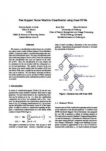
3.2. CUDA Nvidia provides a programming environment for its GPUs called the Compute Unified Device Architecture (CUDA). The user codes in annotated C++, accelerating compute intensive portions of the application by executing them on the GPU. Figure 1 illustrates how the GPU appears to the programmer. The programmer organizes the computation into grids, which are organized as a set of thread blocks. The grids run sequentially on the GPU, meaning that all computation in the grid must finish before another grid is invoked. As mentioned, grids contain thread blocks, which are batches of threads that execute together, sharing local memories and synchronizing at programmer specified barriers. A maximum of 512 threads can comprise a thread block, which puts a limit on the scope of synchronization and communication in the computation. However, enormous numbers of blocks can be launched in parallel in the grid, so that the total number of threads that can be launched in parallel is very high. In practice, we need a large

Fast Support Vector Machine Training and Classification on Graphics Processors

Grid Block (0, 0) Shared Memory Register s

Thread (0, 0) Local Memory

Host

Register s

Thread (1, 0) Local Memory

Block (1, 0) Shared Memory Register s

Thread (0, 0) Local Memory

Register s

Thread (1, 0)

number of training points in the data set: for each data point, an element of f 0 must be computed, which is done by a dedicated thread. After the map function has been performed, the results are summarized by the reduction to compute the final result. In order to extract maximum parallelism, we structure the reduction as a tree, where the number of elements still participating in the reduction halves at each level of the reduction.

Local Memory

Global Memory

Map + Local Reduce

Constant Memory Texture Memory

Figure 1. Logical organization of the GeForce 8800

number of thread blocks to ensure that the compute power of the GPU is efficiently utilized.

4. SVM Training Implementation Since GPUs need a large number of threads to efficiently exploit parallelism, we create one thread for every data point in the training set. The task of each thread is to compute f 0 in (4), which reflects the impact of the optimization step on the optimality conditions of the remaining data points. We then apply the first order working set selection heuristic (Keerthi et al., 2001) to select the points to optimize in the next iteration. The details are explained in the following section.

Global Reduce Figure 2. Structuring the Map Reduce

Because the CUDA programming model has strict limitations on synchronization and communication between thread blocks, we have organized the reduction in stages, as shown in figure 2. The first stage does the map computation, as well as a local reduce within a thread block. Subsequent stages implement the global reduce. Each stage of this process is implemented as a call to the GPU. For really large datasets, the global reduce is done in stages, with more than one call to the GPU. 4.2. Implementation Details

4.1. Map Reduce

4.2.1. Caching

At least since the LISP programming language, programmers have been mapping independent computations onto partitioned data sets, using reduce operations to summarize the results. Recently, Google proposed a Map Reduce variant for processing large datasets on compute clusters (Dean & Ghemawat, 2004). This algorithmic pattern is very useful for extracting parallelism, since it is simple to understand, and maps well to parallel hardware, given the inherent parallelism in the map stage of the computation.

Since evaluating the kernel function Φ(·) is a dominant part of the computation, it is useful to cache as much as possible from the matrix of kernel function evaluations Kij = Φ(xi , xj ) (Joachims, 1999). We compute rows of this matrix on the fly, as needed by the algorithm, and cache them in the available memory on the GPU.

The Map Reduce pattern has been shown to be useful for many machine learning applications (Chu et al., 2007), and is a natural fit for our SVM training algorithm. The computation of f 0 in (4) is the map function, and the search for blow , bhigh , Ilow and Ihigh is the reduction operation. The parallelism needed for extracting performance on the GPU comes from the

When updating the vector f , we need access to two rows of K, since we have changed exactly two entries in α. In our system, the CPU checks to see which of these two rows, if any, are present in the cache. If a row is not present, the CPU voids the least recently used row of the cache, and assigns it to the new row which is needed. For the rows which hit in the cache, the GPU avoids doing the kernel evaluations. Otherwise, the GPU writes out the appropriate row or rows after computing the kernel values.

Fast Support Vector Machine Training and Classification on Graphics Processors

4.2.2. Data Movement

5. SVM Classification Implementation

Programming the GPU requires manually copying data from the host computer to the GPU and vice versa, and it also requires manually copying data from the GPU’s global memory to the fast local stores. As mentioned previously, if the cache does not contain a particular row of K corresponding to the point xj , that row will need to be generated, which means that we need to compute Φ(xi , xj ) ∀i ∈ 1..l. Since the vector xj is shared between all computations, we load it into the GPU’s local store. This is key to performance, since accessing the local store is orders of magnitude faster than accessing the global memory.

We approached the SVM classification problem by making use of the Map Reduce computations as well as vendor supplied Basic Linear Algebra Subroutines - specifically, the Matrix Matrix Multiplication routine (SGEMM), which calculates C 0 = αAB + βC, for matrices A, B, and C and scalars α and β. For the Linear, Polynomial, and Sigmoid kernels, calculating the classification value involves finding the dot product between all test points and the support vectors, which is done through SGEMM. For the Gaussian kernel, we use the simple identity ||x − y||2 = x·x+y·y−2x·y to recast the computation into a Matrix Matrix multiplication, where the SGEMM computes Dij = −γ||zi − xj ||2 = 2γ(zi · xj ) − γ(zi · zi + xj · xj ), for a set of unknown points z and a set of support vectors x. We then apply a map reduce computation to combine the computed D values to get the final result.

4.3. Related Work There have been previous attempts to parallelize the SVM training problem. The most similar to ours is (Cao et al., 2006), which parallelizes the SMO algorithm on a cluster of computers using MPI. Both our approach and their approach use the parallelism inherent in the KKT condition updates as the major source of parallelism. However, in terms of implementation, GPUs present a completely different model than clusters, and hence the amount of parallelism exploited, such as the number of threads, granularity of computation per thread, memory access patterns, and data partitioning are very different. Many other approaches for parallelizing SVM training have been presented. The cascade SVM (Graf et al., 2005) is another proposed method for parallelizing SVM training on clusters. It uses a method of divide and conquer to solve large SVM problems. (Zanni et al., 2006) parallelize the underlying QP solver using Parallel Gradient Projection Technique. Work has been done on using a parallel Interior Point Method for solving the SVM training problem (Wu et al., 2006). (Collobert et al., 2002) proposes a method where the several smaller SVMs are trained in a parallel fashion and their outputs weighted using a Artificial Neural Network. (Ferreira et al., 2006) implement a gradient based solution for SVM training, which relies on data parallelism in computing the gradient of the objective function for an unconstrained QP optimization at its core. Some of these techniques, for example, the training set decomposition approaches like the Cascade SVM are orthogonal to the work we describe, and could be applied to our solver. We implemented the parallel SMO training algorithm because of its relative simplicity, yet high performance and robust convergence characteristics.

Continuing the Gaussian example, the map function exponentiates Dij element wise, multiplies each column of the resulting matrix by the appropriate yj αj . The reduce function sums the rows of the matrix and adds b to obtain the final classification for each data point as given by equation (5). Other kernels require similar map reduce calculations to finish the classification.

6. Results The SMO implementation on the GPU is compared with LibSVM, as LibSVM uses Sequential Minimal Optimization for SVM training. We used the Gaussian kernel in all of our experiments, since it is widely employed. 6.1. Training We tested the performance of our GPU implementation versus LibSVM on the following datasets: Table 3. Dataset Size Dataset Adult Web MNIST USPS Forest Face

# Points 32,561 49,749 60,000 7,291 561,012 6,977

# Dimensions 123 300 784 256 54 381

Adult dataset (Asuncion & Newman, 2007) presents the task of classifying if a person’s income exceeds $50000/year based on census data. Each data-

Fast Support Vector Machine Training and Classification on Graphics Processors Table 4. Details from SVM training on the GPU and with LibSVM

Dataset

# SV

Adult Web MNIST USPS Forest Face

18,666 35,220 43,731 684 270,373 3,310

GPU Iterations 115,838 81,721 68,008 7,062 2,064,502 6,024

point has 123 binary attributes. For this dataset, we used a value of C = 100 and γ=0.5. Web dataset (Platt, 1999) has a set of 300 binary attributes for every point in the dataset. These correspond to the attributes of a web page and the task is to decide if the web page belongs to a particular category or not. C=64 and γ=7.8125 were used (Cao et al., 2006). MNIST dataset (LeCun et al., 1998) has a set of 28×28 images, each of which has a handwritten digit. The task is to be able to classify a digit as one of the 10 categories. Since this is a multiclass classification problem, we converted it into a 2-class problem by doing a even-Vs-odd digit classification. The values of C and γ used were 10 and 0.125 respectively. USPS dataset (Hull, 1994) is also a handwritten digit classification dataset on 12×12 images. An even-Vs-odd classification was performed on the dataset. C=10, γ = 2−8 were used. Forest cover type (Asuncion & Newman, 2007) is a dataset of cartographic variables from US Geological survey data. The task is to predict forest cover type from the information. It is a multiclass classification problem. We have used a class-2-versus-the-rest problem for our experiments. C=10 and γ=0.125 were used. Face detection dataset (Rowley et al., 1998) has a set of 19×19 images of faces and non-faces, which are histogram equalized and normalized. The task is to separate the faces from the non-faces. The training values used were C=10 and γ=0.125. The sizes of the datasets are given in table 3. We ran LibSVM on an Intel Core 2 Duo 2.66 GHz processor, and gave LibSVM a cache size of 650 MB, which is slightly larger than our GPU implementation was allowed. File I/O time was not included in solver

LibSVM # SV Iterations 19,058 35,232 43,756 684 270,311 3,322

43,735 85,299 76,385 4,614 275,516 5,342

% difference in b 0.006 0.01 0.04 0.02 0.08 0.01

runtime. Table 4 shows results from our solver. Since any two solvers give slightly different answers on the same optimization problem, due to the inexact nature of the optimization process, we show the number of support vectors returned by the two solvers as well as how close the final values of b were for the GPU solver and LibSVM, which were both run with the same tolerance value τ = 0.001. As shown in the table, the deviation in number of support vectors between the two solvers is less than 2%, and the deviation in the offset b is always less than 0.1%. Our solver provides equivalent accuracy to the LibSVM solver, which will be shown again in the classification results section. Table 5. Comparison of GPU vs LibSVM solve times Dataset Adult Web MNIST USPS Forest Face

GPU (sec) 36.312 181.334 525.783 0.733 13360.785 2.57

LibSVM (sec) 550.178 2422.469 16965.794 5.092 66523.538 27.61

Speedup 15.1 13.4 32.3 6.9 5.0 10.7

Table 5 contains performance results for the two solvers. We see speedups in all cases from 5× to 32×. There is still room for improving these figures, since we have not yet implemented all the optimizations possible for this problem. For example, LibSVM uses a second order heuristic for picking the new points for doing a single iteration of QP optimization, while our GPU implementation uses a first order heuristic. In most cases, this leads to the GPU solver running many more iterations than LibSVM. Also, for large sparse datasets, our solver is disadvantaged because we currently represent the data in a dense format. Furthermore, we haven’t yet implemented working set shrinking. Despite the relative immaturity of our solver, we still achieve significant performance gains. For problems with large dimensions and where the number of iterations are close to those of LibSVM, the GPU solver achieves significant speedups.

Fast Support Vector Machine Training and Classification on Graphics Processors Table 6. Performance and accuracy of GPU SVM classification vs. LibSVM

Dataset Adult Web MNIST USPS Face

GPU Accuracy Time (s) 6619/8000 0.570 3920/4000 1.069 2400/2500 1.98 1948/2007 0.0097 23664/24045 0.706

6.2. Classification Results for our classifier are presented in table 6. We achieve 120-150x speedup over LibSVM on the datasets shown. As with the solver, file I/O times were excluded from overall runtime. When performing the classification tests, we used the SVM classifier output by the GPU solver with the GPU classifier, and used the SVM classifier provided by LibSVM’s solver to perform classification with LibSVM. Thus, the accuracy of the classification results presented in table 6 reflect the overall accuracy of the GPU solver and GPU classifier system. The results are essentially identical. Only one out of 40552 test points were classified differently between the two systems, which shows that our GPU based SVM system is as accurate as traditional CPU based methods.

7. Conclusion This work has demonstrated the utility of graphics processors for SVM classification and training. Training time is reduced by 5 − 32×, and classification time is reduced by 120 − 150× compared to LibSVM. These kinds of performance improvements can change the scope of SVM problems which are routinely solved, increasing the applicability of SVMs to difficult classification problems. For example, finding a classifier for an input data set with 60000 data points and 784 dimensions takes less than ten minutes on the GPU, compared with almost 5 hours on the CPU. Scanning images for faces with SVMs can be done at a rate of 34200 Faces/second versus only 220 Faces/second on the CPU. The GPU is a very low cost way to achieve such high performance: the GeForce 8800 GTX fits into any modern desktop machine, and currently costs $500, while the compatible GeForce 8800 GT provides 97% of the floating-point performance for only $300. Problems which used to require a compute cluster can now be solved on one’s own desktop. New machine learning algorithms that can take advantage of this kind of performance, by expressing parallelism widely, will

LibSVM Accuracy Time (s) 6619/8000 75.65 3920/4000 144.53 2400/2500 258.751 1948/2007 1.194 23665/24045 109.259

Speedup 132.5 135.2 130.7 123.2 154.8

provide compelling benefits on future many-core platforms.

References Asanovi´c, K., Bodik, R., Catanzaro, B. C., Gebis, J. J., Husbands, P., Keutzer, K., Patterson, D. A., Plishker, W. L., Shalf, J., Williams, S. W., & Yelick, K. A. (2006). The Landscape of Parallel Computing Research: A View from Berkeley (Technical Report UCB/EECS-2006-183). EECS Department, University of California, Berkeley. Asuncion, A., & Newman, D. (2007). UCI machine learning repository. Cao, L., Keerthi, S., Ong, C.-J., Zhang, J., Periyathamby, U., Fu, X. J., & Lee, H. (2006). Parallel sequential minimal optimization for the training of support vector machines. IEEE Transactions on Neural Networks, 17, 1039–1049. Chu, C.-T., Kim, S. K., Lin, Y.-A., Yu, Y., Bradski, G., Ng, A. Y., & Olukotun, K. (2007). Map-reduce for machine learning on multicore. In B. Sch¨ olkopf, J. Platt and T. Hoffman (Eds.), Advances in neural information processing systems 19, 281–288. Cambridge, MA: MIT Press. Collobert, R., Bengio, S., & Bengio, Y. (2002). A parallel mixture of svms for very large scale problems. Neural Computation, 14, 1105–1114. Cortes, C., & Vapnik, V. (1995). Support-vector networks. Mach. Learn., 20, 273–297. Dean, J., & Ghemawat, S. (2004). Mapreduce: simplified data processing on large clusters. OSDI’04: Proceedings of the 6th Symposium on Operating Systems Design & Implementation. Berkeley, CA, USA: USENIX Association. Fan, R.-E., Chen, P.-H., & Lin, C.-J. (2005). Working set selection using second order information for training support vector machines. J. Mach. Learn. Res., 6, 1889–1918.

Fast Support Vector Machine Training and Classification on Graphics Processors

Ferreira, L. V., Kaskurewicz, E., & Bhaya, A. (2006). Parallel implementation of gradient-based neural networks for svm training. International Joint Conference on Neural Networks. Graf, H. P., Cosatto, E., Bottou, L., Dourdanovic, I., & Vapnik, V. (2005). Parallel support vector machines: The cascade svm. In L. K. Saul, Y. Weiss and L. Bottou (Eds.), Advances in neural information processing systems 17, 521–528. Cambridge, MA: MIT Press. Hull, J. J. (1994). A database for handwritten text recognition research. IEEE Trans. Pattern Anal. Mach. Intell., 16, 550–554. Joachims, T. (1999). Making large-scale support vector machine learning practical. In Advances in kernel methods: support vector learning. Cambridge, MA, USA: MIT Press. Keerthi, S. S., Shevade, S. K., Bhattacharyya, C., & Murthy, K. R. K. (2001). Improvements to Platt’s SMO Algorithm for SVM Classifier Design. Neural Comput., 13, 637–649. LeCun, Y., Bottou, L., Bengio, Y., & Haffner, P. (1998). Gradient-based learning applied to document recognition. Proceedings of the IEEE, 86, 2278–2324. Nvidia (2007). Nvidia CUDA. http://nvidia.com/ cuda. Osuna, E., Freund, R., & Girosi, F. (1997). An improved training algorithm for support vector machines. Neural Networks for Signal Processing [1997] VII. Proceedings of the 1997 IEEE Workshop, 276– 285. Platt, J. C. (1999). Fast training of support vector machines using sequential minimal optimization. In Advances in kernel methods: support vector learning, 185–208. Cambridge, MA, USA: MIT Press. Rowley, H. A., Baluja, S., & Kanade, T. (1998). Neural network-based face detection. IEEE Transactions on Pattern Analysis and Machine Intelligence, 20, 23–38. Wu, G., Chang, E., Chen, Y. K., & Hughes, C. (2006). Incremental approximate matrix factorization for speeding up support vector machines. KDD ’06: Proceedings of the 12th ACM SIGKDD international conference on Knowledge discovery and data mining (pp. 760–766). New York, NY, USA: ACM Press.

Zanni, L., Serafini, T., & Zanghirati, G. (2006). Parallel software for training large scale support vector machines on multiprocessor systems. J. Mach. Learn. Res., 7, 1467–1492.