Fast Toggle Rate Computation for FPGA Circuits - EECG Toronto

FAST TOGGLE RATE COMPUTATION FOR FPGA CIRCUITS Tomasz S. Czajkowski Department of ECE, University of Toronto, Toronto, Ontario, Canada [email protected] ABSTRACT This paper presents a fast and scalable method of computing signal toggle rate in FPGA-based circuits. Our technique is a vectorless estimation technique, which can be used in a CAD tool to identify the parts of the circuit that can benefit from power optimization. A key advantage of our approach is its ability to efficiently account for spatial correlation of related logic cones, which is accomplished using a novel XOR-based decomposition. In addition, our approach uses post-routing circuit delays to account for glitches in a logic circuit. The proposed approach was tested on 14 MCNC benchmark circuits compiled for the Altera Stratix II devices. The results indicate that our method improves the vectorless estimation technique available in the latest version of Altera’s Quartus II commercial CAD tool, reducing the average error by 37% and standard deviation by 59%. 1. INTRODUCTION Field-Programmable Gate Array (FPGA) devices are a popular choice for low to medium volume digital applications. They can implement various different circuits without a need to fabricate a new chip, reducing costs and time to market. This flexibility is paid for by increased power dissipation. The power consumed by a circuit implemented on an FPGA device in a 90nm process, or smaller, presents a problem, especially if an FPGA device is to be used in a mobile application. The power dissipation of a 4-input LUT based FPGA consists 40% of static power and 60% of dynamic power, with static power increasing with shrinking feature sizes and increasing LUT sizes [3]. The dynamic power dissipation is determined by the toggle rate of signals in the circuit, which can as much as double when glitches are present [2]. Several works that address the topic of toggle rate estimation already exist [1][2][4][6-13]. In the work on transition density [1] the toggle rate is represented using the theory of probability. The main advantage of this approach is that toggle rate can be represented using statistical analysis, producing reasonably accurate results for the overall power dissipation in a logic circuit. However, the accuracy of results on a per connection basis is low, preventing power reduction algorithms from effectively optimizing a logic circuit. The work in [2] looks at the transition density (average number of times a signal toggles per unit time) [1] and how

Stephen D. Brown Department of ECE, University of Toronto, Toronto, Ontario, Canada [email protected] this concept applies to circuits implemented on FPGAs. The transition density is represented as a weighted sum of transitions generated and propagated through a LUT. The generated transitions are a function of LUT depth and the number of paths to LUT inputs. Propagated transitions are due to glitches that propagate through a LUT and are based on the logic function the LUT implements. The work in [2] was intended to predict the toggle rate of a circuit before it is placed and routed. The work in [4] focuses on transition density computation once circuit delays are known. Their approach is in essence an event driven simulation, except that logic transitions are represented using a probabilistic waveform. This method effectively combines multiple events on primary inputs of a circuit into a single probabilistic waveform to obtain transition density values. A probabilistic model introduced in [7] accounts for both temporal and spatial correlation in a circuit. Using ROBDDs to perform correlation analysis improved the computation time of their method, and the approach scales much better in terms of processing time than competing approaches presented in [8] and [13]. Unfortunately, the method only computes the static and transition probabilities, ignoring glitches caused by delay imbalance in a circuit. In FPGA circuits such glitches can cause the number of transitions on any given wire to double [2], resulting in an increased power dissipation. Hence, a toggle rate analysis method needs to account for glitching as well as correlation of logic signals. This work presents a fast approach to compute toggle rate on a per wire basis using an XOR-based logic decomposition. It considers temporal and spatial correlations, as well as glitching of logic signals due to delay imbalance in a logic circuit. The proposed approach processes the circuit in topological order computing transition density for each LUT. For LUT inputs that are correlated, the approach performs a Gaussian Elimination based decomposition. It first determines the cones of logic that capture the dependency between these inputs and then decomposes these cones into subfunctions that expose the correlation between them in an efficient manner. The decomposition is then used to account for spatial correlation of LUT inputs. The approach was tested on several MCNC benchmarks as well as several industrial benchmarks, targeting the Altera Stratix II FPGA. The results show a significant improvement of the approach currently available in the most recent release of Quartus II. The remainder of this paper is organized as follows:

Section 2 contains background information. Section 3 describes our toggle rate analysis method, focusing on temporal and spatial correlation. The equations used to compute correlation are derived in Section 4, while the experimental results are presented in Section 5. The conclusion and avenues for further research are in Section 6. 2. BACKGROUND The average dynamic power dissipation of a logic circuit is defined by the following equation:

Pavg =

∑ ( fi CiV 2 )

(1)

all nets i

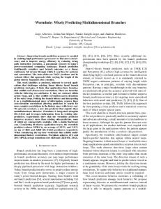
where fi is the transition density measured on a per second basis, Ci is the net capacitance, and V is the power supply voltage. In a circuit where the primary inputs are registered, we can expand fi as si*fclock, where fclock is the clock frequency and si is the per cycle transition density of a net. The transition density is a key parameter in this equation as it changes depending on the logic function of a component that drives it, as well as logic functions in its transitive fanin, logic and wire delays, as well as glitches. The computation of transition density involves the use of several parameters: static probability, 061 transition probability and 160 transition probability. Static probability defines the likelihood that a logic signal is at a logic value of 1. The 061 transition probability determines how likely a signal is to change state once it is at a logic 0 value. Similarly, the 160 transition probability accounts for the likelihood of a signal changing state when it is at a logic 1 value. The latter two parameters are commonly referred to as the temporal correlation of a signal. While these three parameters are necessary to compute transition density for any given logic function, each of them is affected by what is known as spatial correlation [5]. Spatial correlation is a measure of the relationship between logic signals at an input of a logic gate. This occurs when logic expressions for each of the inputs are related by common set of signals, either primary inputs or an internal signal. In both cases a particular logic state of one input affects the static probability of the other inputs. To compute spatial correlation for any given set of gate inputs, it is important to be able to quickly determine the nature of the relationship between these signals. To do this, we utilize an XOR-based logic decomposition based on Gaussian Elimination. The basic idea behind this decomposition is demonstrated on the example in Figure 1. Figure 1 shows a simple logic function of four variables. We can see that each column of the truth table is different from the others, however a close inspection reveals that column 11 is an XOR of columns 01 and 10. By utilizing this fact we can extract two logic sub functions, G1=c to represent column 01 and G2=d to represent column 10. Column 11 would therefore be G1rG2, allowing the overall function to

ab 00 01 10 11

cd 00 01

0 0

0 0

0 1

0 1

10 11

0 0

1 1

0 1

1 0

Fig. 1. Decomposition using Gaussian Elimination be synthesized as f=bG1raG2=bcrad. The problem of finding such relationships between logic columns is solved by using Gaussian Elimination. By utilizing Gaussian Elimination along with BDDs the approach can be effectively applied to large circuits and the synthesis of multi-output functions [14]. 3. TOGGLE RATE COMPUTATION The computation of the toggle rate of a logic signal in an FPGA circuit consists of two components - transitions generated by a LUT and glitches propagated from LUT inputs to its output. The transitions generated by a LUT are those that occur due to changes in logic state of LUT inputs. If LUT inputs change at different times, then glitches may be generated. For example, a 3-LUT with inputs a, b, and c can produce two intermediate values while its inputs change from input pattern 000 to 111. Thus if the LUT produces a logic 0 for inputs 000, logic 1 for 001, logic 0 for 011 and logic 1 for inputs 111, then the LUT output will show 3 transitions, whereas only one should occur. Furthermore, these glitches may be propagated by LUTs downstream. Transitions due to glitches would occur on top of the transitions generated by a LUT and should be added to the toggle rate for a given LUT output. In the following explanations we utilize the concept of transition density to express the toggle rate, measuring transitions on a per clock cycle basis. 3.1 Basic Approach The basic approach is to process each LUT one at a time in a topological order. For each LUT, we evaluate the static probability, transition probability, transition density, 061 and 160 transition probabilities and use them in computations downstream. This is done by computing transitions generated by, and propagated through, a LUT. Transitions generated by a LUT are computed using the static probability for each possible input valuation, the probability of transition from one valuation to another, and the arrival time of each signal at a LUT input. The transition density generated by a LUT is computed as follows: 1..1

Dg =

1..1

∑ ∑ ( P [i ] P  j i  Trans(i, j) )

(2)

i = 0..0 j = 0..0

where i and j represent input valuations, and P[i] is the static probability of a given input valuation, P[j|i] is the probability

that inputs change from pattern i to j and Trans(i,j) is the number of transitions generated when input pattern changes from i to j. The last term uses the arrival time of each input signal to determine the number of transitions that will occur at the output of a LUT by changing input pattern i to j one bit at a time in the order determined by their arrival time. Now that the generated transitions are accounted for, we need to compute the transition density component due to glitches propagated through a LUT. To account for the glitches we utilize the concept of Boolean Difference in a fashion similar to [1]. However, we impose a constraint on glitch forwarding such that the glitches from an input x of a LUT are forwarded to its output only during such input transitions that both the initial and the final input valuations are sensitive to changes on input x. Because of this restriction, we need to account for the probability of a particular input transition in the same manner as in Equation 2. Thus, the probability glitches on input x are transferred to the LUT output is computed as follows: df (i ) df ( j ) Pfx ( i, j ) = * * P [i ] * P  j i  (3) dx dx where f is the function implemented by the LUT and df/dx is the Boolean Difference of f with respect to LUT input x. The above equation will be equal to P[i]P[j|i] only when both the initial (i) and final (j) input valuations cause function f to change value if input x changes value (df/dx=1). Otherwise, the equation will evaluate to 0, signifying that glitches from input x will not propagate to the LUT output during the specified transition. Using this definition we can express the transition density due to glitching on a LUT input x as: 1..1

Dp ( x ) =

1..1

∑ ∑ ( Pfx ( i, j ) *  D ( x ) − Pt ( x ) )

(4)

i = 0..0 j = 0..0

where Pt(x) is the transition probability of input x and D(x)Pt(x) is the average number of glitches per cycle on input x. Using the above approach we can define the total transition density for any given wire y as: n

D ( y ) = Dg + ∑ D p ( xi )

(5)

i =1

While the above computation is relatively simple, its key parameters (P[i] and P[j|i]) are affected by correlation [5]. 3.2 Temporal Correlation The temporal correlation describes the behaviour of a logic signal with respect to its previous value. It is defined by the 061 and 160 transition probabilities. These probabilities determine how likely a signal is to change state given its present state. For example, a signal that assumes a logic value 1 for a single clock cycle once every 8 cycles on average, would have a 061 transition probability of 1/8, while its 160 transition probability would be equal to 1. In our model these probabilities affect the P[j|i] parameter, which determines the likelihood of a transition from one state to another.

b a c

h f g

d Fig. 2. Correlated logic cones g and h are used as inputs to an AND gate, forming function f. 3.3 Spatial Correlation The spatial correlation is a more complex type of correlation observed in logic circuits. It is important because it can change both the probability of any given input pattern as well as the probability of input transition. The basic idea behind spatial correlation is that two, or more, signals may share logic in their transitive fanin. As such, their logic state can be related to a varying degree. An extreme example is one where two inputs, x and y, are related by inversion, in which case neither xy=00 nor xy=11 are possible input valuations. Similarly, the spatial correlation may change the probability of input transition. For example, suppose that two inputs to a LUT, x and y, were related in such a way that when y=1 then x must equal 1, otherwise x can be either 0 or 1. In such a case we know that transition from xy=11 to xy=01 is not possible. In our approach we utilize a fast logic decomposition to efficiently compute spatial correlation. The use of a fast decomposition in our approach makes it possible to speed up the computation of correlation by looking at a collection of small logic functions, rather than a few large ones. While many decompositions exists, [14] has been shown to be efficient in handling reasonably large logic functions. To demonstrate our approach consider the example in Figure 2. It shows an example of a logic circuit, where the right-most AND gate f depends on two logic functions, g and h, that have the same support. We now show how [14] is used to compute conditional probability of g given h, allowing us to account for correlation of these two logic functions during toggle rate analysis of the AND gate producing signal f (encircled gate in Figure 2). Figure 3 shows our initial setup, where logic functions for g and h are put side by side and variables a and b are assigned to the rows of the combined truth table. With this setup in place we apply the decomposition in [14] to find their common subfunctions. They are X1=a and X2=b. The selector functions for X1 and X2 in function g are Sg1=!(cd) and Sg2=d. Given this decomposition, our goal is to determine the conditional probability P[g=1 | h=1]. The basic idea of the following computation is to determine how each of the subfunctions, X1 and X2, that cause function g to assume a logic value 1 are affected by the logic state of function h. To do so we first compute when

g

benchmarks neither constraint is needed due to a relatively small number of inputs, it has been imposed to handle large circuits where the total number of primary inputs exceeds 24.

h

cd

cd

00 01 10 11 00 01 10 11 00 0 0 0 0 0 0 0 0 ab 01 10 11

0 1 1

1 1 0

0 1 1

1 0 1

1 0 1

0 1 1

0 1 1

0 1 1

Fig. 3. Truth tables for functions g and h. X1S1 h cd cd 00 01 10 11 00 01 10 11 00 0 0 0 0 0 0 0 0 ab 01 0 0 0 0 1 0 0 0 10 1 1 1 0 0 1 1 1 11 1 1 1 0 1 1 1 1 Fig. 4. Correlation between X1S1 and h both X1S1 and h are both at a logic value 1 and the probability of such event. This is illustrated in Figure 4. In Figure 4 the indicated truth table entries on the left side are the 1s in X1S1 that appear in the same position as 1s in function h. Therefore, for 5 of 8 ones in function h, X1S1 has a corresponding logic 1 entry. Thus, if inputs a, b, c, and d have static probability of ½ and are independent then we can see that P[X1S1 | h] = 5/8. In a similar manner we can determine that P[X2S2 | h] = 2/8. Now that the simple cases are covered, it is important to account for the fact that both X1S1 and X2S2 could be 1 for the same pattern of inputs a, b, c, and d. In our example this happens for abcd=1101. To account for this difference we need to subtract this event from our final result. More formally, we need to subtract 2P[X1S1X2S2 | h], because in this case function g is equal to 0 as a result of using an XOR decomposition. The factor of 2 is also imposed because this event was first included when computing P[X1S1 | h] and then again when computing P[X2S2 | h]. After accounting for the above terms we find P[g=1 | h=1] to be equal to 5/8+2/8-2/8=5/8, which we can confirm is the correct result by inspection of Figure 3. In a similar manner we can compute P[g=1 | h=0] and thereby have enough information to describe the relationship between static probabilities of these two logic functions. The above explains how we adjust static probability for any state of inputs of a LUT, but it does not describe how we choose the cones of logic for each input of a LUT. In that respect our approach is consistent with [7] as we only look at logic up to a certain depth. While in [7] a depth of up to 10 logic gates was used, we utilize a constraint on reconvergent fanout to be within a depth of 4 LUTs and that the cone of logic does not exceed 24 inputs. While in some of the MCNC

4. COMPUTING SPATIAL CORRELATION In this section we derive equations that we use to determine correlation between logic signals, taking into account the method in which the logic cones were decomposed. The derivation begins with Bayes’ rule: P [ g ∩ h] P  g h  = (6) P [h] What is needed now is the computation of P[g1h]. The first step is to expand g as an XOR of products of X1..n and S1..n:    P [ g ∩ h ] = P  X i Si  ∩ h  (7)   i   While we cannot separate XiSi and h, we can include h within the summation. Doing so allows us to expand the probability of this expression into a sum of probabilities: P [ g ∩ h] = P  X i Si ∩ h  −

∑

∑ i

2∑ i

4∑ i

∑ P  X i X j Si S j ∩ h  + j = i +1

∑ ∑

(8)

P  X i X j X k Si S j Sk ∩ h  − ...

j =i +1 k = j +1

A similar derivation is used to expand P[XiSi 1 h] terms with respect to function h. When h is expanded, the resulting expression is a product of basis and selector functions for g and h. Since basis functions have disjoint support from selector functions, then the probability computation is simplified to the product of probabilities of two logic functions. One function has the support the same as the basis functions, while the other includes the support of the selector functions for both g and h. In the above derivation, functions Xi and Si have disjoint support and therefore are assumed to be independent. While this assumption may not always hold and we will see errors as a results, to assume otherwise means using logic functions as a function of primary inputs of a circuit, which for all practical purposes is not feasible. However, as we will show through our results, the estimation error is acceptable. 5. EXPERIMENTAL RESULTS We conducted experiments to evaluate the effectiveness and processing time of the proposed approach on 14 MCNC circuits implemented on the Altera Stratix II FPGA. We used ModelSIM-Altera 6.0c and 10000 random vectors to generate the reference toggle rate for each benchmark circuit. We then ran the Quartus II 7.1 PowerPlay Power Analyzer to determine the actual toggle rate of each wire, accounting for inertial delay [1] that would cause some glitches not to

Table 1. Toggle Rate Estimation Results in Comparison to Quartus II 7.1. Circuit alu4 apex2 apex4 C2670 C3450 cps dalu ex5p ex1010 misex3 pair pdc seq spla Average

ALUTs 731 797 645 117 262 427 193 504 1802 732 336 1894 854 1495

Quartus II 7.1 Average Error (%)

Quartus II 7.1 St. Dev.

Our Average Error (%)

Our St. Dev.

23.33 55.82 22.01 -8.84 -8.04 30.33 20.31 10.25 7.88 29.80 -2.07 15.25 44.55 30.84

58.39 55.26 74.74 22.56 45.56 68.13 53.98 76.24 83.62 64.54 32.10 82.31 60.92 76.49

0.30 -2.03 -14.65 -1.51 -12.12 -0.14 -8.50 -6.53 -25.47 -8.06 -2.93 -26.57 -3.07 -24.13 -9.67

22.37 29.49 20.15 16.10 20.83 40.26 20.59 22.00 21.73 22.09 11.43 25.12 33.34 23.80 23.52

appear on a wire. 5.1 Experimental Procedure and Results To generate results we used the transition density and static probability values from simulation to define the behaviour of the primary inputs of each circuit. We then applied our technique to estimate the toggle rate of each benchmark circuit and compared it to the results obtained via simulation. We also applied the vectorless toggle rate estimation technique available in Quartus II 7.1 to the benchmark suite to see how our method fairs in comparison to one currently used in FPGA industry. The input to the Quartus II 7.1 Power Play Power Analyzer was the same as to our approach. In both cases we compared the estimate to the actual toggle rate for each wire using the following formula: (estimated − actual ) %diff = 100 * (9) MAX (estimated , actual ) We used the result for each wire in a circuit to determine the average percentage error as well as standard deviation for the error distribution. The results are shown in Table 1. In Table 1 each circuit is listed by name in the left column. In column 2 we list the size in terms of ALUTs the circuit occupied on the Altera Stratix II FPGA. Columns 3 and 4 show the average error and standard deviation for toggle rate prediction made by Quartus II 7.1. In columns 5 and 6 we show the average error and standard deviation for our toggle rate prediction method. In column 7 we show the processing time needed for our approach to analyze toggle rate of each circuit. Finally, in column 8 we compare average error magnitude as computed by our method to Quartus II 7.1, while in column 9 we compare the standard deviation to that obtained by Quartus II 7.1. 5.2 Discussion Our toggle rate estimation technique was able to achieve a 9.67% average error with a standard deviation of 23.52%.

Our Processing Time (s) 3 2.9 2.7 0.7 1.5 1.4 1.1 3.6 31.2 2.8 1.9 30.7 3.4 21.4

Average Error Our vs. Quartus II 7.1 (%) -98.71 -96.36 -33.44 -82.92 33.66 -99.54 -58.15 -36.29 69.06 -72.95 29.35 42.60 -93.11 -21.76 -37.04

St. Dev. Our vs. Quartus II 7.1 (%) -61.69 -46.63 -73.04 -28.63 -54.28 -40.91 -61.86 -71.14 -74.01 -65.77 -64.39 -69.48 -45.27 -68.88 -59.00

While there is room for improvement, the approach proved to be computationally efficient, where the processing time as a function of circuit size grows at a reasonable rate. In most cases our approach was able to achieve a very good average error. It was particularly effective in cases where the circuit had a large number of inputs, where expressing LUT inputs in terms of primary circuit inputs was not a viable alternative. Examples of such circuits were C2670 and pair. Other circuits for which the average estimate error was low had few levels of LUTs and a low number of primary inputs. An example of such a case is alu4 and cps. For such circuits capturing the reconvergent fanout within 4 levels of ALUTs was sufficient to either incorporate primary inputs in the computation, or capture enough of the correlation to compute the toggle rate effectively. This was not the case in three of our circuits, namely ex1010, pdc and spla. Each of those circuits has at most 16 primary inputs. However, what these circuits lack in the number of inputs they make up for in the number of logic levels required to compute the final result. As such, our approach of looking at 4 ALUT levels was insufficient to capture the spatial correlation, though exploring more levels would have lead to encompassing all primary inputs in the computation and producing a better result. Such approach, however, would not have worked well in circuits with larger number of inputs, as the processing time and the cone sizes would be large. In addition to average error we are providing a standard deviation to show the consistency of our results. On average the standard deviation of the toggle rate prediction error is 23.52%. While this may seem large, the question becomes how significant this error is in terms of absolute estimate error. To determine this we analyzed absolute toggle rate error for the MCNC circuits to find out the magnitude of the error we can expect with our approach. The graph in Figure 5 shows absolute estimate error achieved by our approach.

could be compressed. This could speed up the correlation computation and allow the cone sizes to be much larger, thereby improving the accuracy of results. 7. ACKNOWLEDGMENTS The authors would like to thank Dr. D. Lewis for feedback during the course of this work. We also appreciate the assistance of Dr. A. Grbic and B. Chan with running experiments using Quartus II software. We thank Altera Corporation for funding this research. 8. REFERENCES Fig. 5. Absolute Estimation Error histogram The average error of the distribution shown in Figure 5 is 0.024 transitions per cycle and the standard deviation is 0.085 transitions per cycle. 5.3 Related Work The work closest to ours is [7]. The work presented there uses BDDs to compute correlation between logic signals, and similarly to our approach create cones of logic up to a certain depth to capture spatial correlation. The main differences between the approach in [7] and ours is the use of logic decomposition to speedup toggle rate computation as well as the use of post-routing delay data to account for glitches. In contrast to the work in [2], which also accounts for the presence of glitches, our approach uses the logic equation of a LUT to compute the transition density generated by a LUT and does not require calibration to work well with any given CAD tool. Instead, it depends only on device parameters, such as logic and interconnect delays, and inertial delay [1]. 6. CONCLUSION AND FUTURE WORK This paper presented a new approach to toggle rate computation that utilizes a fast XOR-based logic decomposition technique [14]. The decomposition technique was chosen because of its ability to quickly compute a functional decomposition of logic functions, even for logic cones that exceed 20 inputs. In contrast, other techniques would require more time to process cones of similar size, or the generated decomposition would consist of larger number of subfunctions than the technique presented in [14]. This helps us provide a better result in a shorter amount of time. The method presented here was applied to circuits implemented on the Altera Stratix II FPGA, showing a significant improvement in the accuracy of toggle rate estimating as compared to the one currently used in the Quartus II commercial CAD tool. A further area of study along the proposed approach is to further compress the data used in correlation computation. The main idea here would be to preserve only the logic nets that are part of the reconvergent paths, while the other nets

[1]

[2]

[3]

[4]

[5]

[6]

[7]

[8]

[9]

[10]

[11]

[12]

[13]

[14]

F. Najm, "Transition Density: a new measure of activity in digital circuits," IEEE Trans. on CAD of Integrated Circuits and Systems, February 1993, Vol. 12, pp. 310-323. J. H. Anderson and F. N. Najm, "Switching Activity Analysis and Pre-Layout Activity Prediction for FPGAs," ACM/IEEE Workshop on SLIP, 2003, pp. 15 - 21. F. Li, D. Chen, L. He, J. Cong, "Architecture Evaluation for Power-Efficient FPGAs," ACM/SIGDA Int. Conf. On FPGAs, 2003, pp.175-184. C. Tsui, M. Pedram and A. M. Despain, "Efficient Estimation of Dynamic Power Consumption under Real Delay Model," IEEE Int. Conf. On CAD, 1993, pp. 224-228. P. H. Schneider and S. Krishnamoorthy, “Effects of Correlations on Accuracy of Power Analysis - An Experimental Study,” Proc. of ISLPD, 1996, pp. 113-116. J. Monteiro, S. Devadas, A. Ghosh, K. Keutzer, and J. White, “Estimation of average switching activity in combinational circuits using symbolic simulation,” IEEE Trans. on CAD, Vol. 16, No. 1, Jan 1997, pp. 121-127. P. H. Schneider, U. Schlichtmann, and B. Wurth, “Fast Power Estimation of Large Circuits,” IEEE Design and Test of Computers, 1996, pp.70-77. R. Marculescu, D. Marculescu, and M. Pedram, “Probabilistic Modeling of Dependencies During Switching Activity Analysis,” in IEEE Trans. on CAD, Vol.12, No.2, Feb. 1998, pp. 73-83. T. Chou and K. Roy, “Accurate Estimation of CMOS Sequential Circuits,” IEEE Trans. on VLSI, Vol.4, No.3, Sept. 1996, pp. 369-380. J. C. Costa, J. C. Monteiro, and S. Devadas, “Switching Activity Estimation Using Limited Depth Reconvergent Path Analysis,” Proc. of ISLPD, 1997, pp. 184-189. G. Theodoridis, S. Theoharis, D. Soudris, and C. Goutis, “Switching Activity Estimation Under Real-Gate Delay Using Timed Boolean Functions,” in IEE Proc. on Computers & Digital Techniques, Vol. 147, No. 6, Nov. 2000, pp. 444-450. F. Hu and V. D. Agrawal, “Dual-Transition Glitch in Probabilistic Waveform Power Estimation,” Proc. of ACM Great Lakes Symposium on VLSI, 2005, pp. 357-360. T. Chou, K. Roy, and S. Prasad, “Estimation of Circuit Activity Considering Signal Correlations and Simultaneous Switching,” IEEE Proc. of ICCAD, 1994, pp. 300-303. T.S. Czajkowski and S.D. Brown, “Functionally Linear Decomposition and Synthesis of Logic Circuits for FPGAs,“ IEEE Proc. of the 45th DAC, 2008, pp. 18-23.