In Section 3, we state and analyze three new .... We define S(n, N) to be the random variable that counts .... The random variable V = 1 - U is uniformly distrib-.
RESEARCHCONTRIBUTIONS
Lloyd Fosdick Guest Editor
Faster Methods for Random Sampling
JEFFREY SCOTT VITTER
ABSTRACT: Several new methods are presented for selecting n records at random without replacement from a file containing N records. Each algorithm selects the records for the sample in a sequential manner--in the same order the records appear in the file. The algorithms are online in that the records for the sample are selected iteratively with no preprocessing. The algorithms require a constant amount of space and are short and easy to implement. The main result of this paper is the design and analysis of Algorithm D, which does the sampling in O(n) time, on the average; roughly n uniform random variates are generated, and approximately n exponentiation operations (of the form ab, for real numbers a and b) are performed during the sampling. This solves an open problem in the literature. CPU timings on a large mainframe computer indicate that Algorithm D is significantly faster than the sampling algorithms in use today. 1. INTRODUCTION Many computer science and statistics applications call for a sample of n records selected randomly without replacement from a file containing N records or for a random sample of n integers from the set {1, 2, 3 . . . . . NI. Both types of random sampling are essentially equivalent; for convenience, in this paper we refer to the former type of sampling, in which records are selected. Some important uses of sampling include market surveys, quality control in manufacturSome of this research was done while the author was consulting for the IBM Pale Alto Scientific Center, Support was also provided in part by NSF Research Grant MCS-81-05324, by an IBM research contract, and by ONR and DARPA under Contract N00014-83.K-0146 and ARPA Order No. 4786. An extended abstract of this research appears in [10].
©1984ACMO001.0782/84/0700-0703 75¢
July 1984 Volume 27 Number 7
ing, and probabilistic algorithms. Interest in this subject stems from work on a new external sorting method called BucketSort that uses random sampling for preprocessing [7]. One way to select the n records is to generate an independent random integer k between I and N and to select the kth record if it has not already been selected; this process is repeated until n records have been selected. (If n > N/2, it is faster to select the N - n records not in the sample.) This is an example of a nonsequential algorithm because the records in the sample might not be selected in linear order. For example, the 84th record in the file may be selected before the 16th record in the file is selected. The algorithm requires the generation of O(n) uniform random variates, and it runs in O(n) time if there is enough extra space to check in constant time whether the kth record has already been selected. The checking can be done in O(N) space using a bit array or with O(n) pointers using hashing techniques (e.g,, [2, 6]}. In either case, the space required may be prohibitive. Often, we want the n records in the sample to be in the same order that they appear in the file so that they can be accessed sequentially, for example, if they reside on disk or tape. In order to accomplish this using a nonsequential algorithm, we must sort the records by their indices after the sampling is done. This requires O(n log n) time using a comparison-based sorting algorithm like quicksort or heapsort; address-calculation sorting can reduce the sorting time to O(n), on the average, but it requires space for O(n) pointers. Nonsequential algorithms thus take nonlinear time, or their space requirements are very large and the algorithm is somewhat complicated.
Communications of the ACM
703
Research Contributions
More importantly, the n records cannot be output in sequential order online: It takes O(n) time to output the first element since the sorting can begin only after all n records have been selected. The alternative we take in this paper is to investigate sequential random sampling algorithms, which select the records in the same order that they appear in the file. The sequential sampling algorithms in this paper are ideally suited to online use since they iteratively select the next record for the sample in an efficient way. They also have the advantage of being extremely short and simple to implement. The measure of performance we use for the algorithms is CPU time, not I / O time. This is reasonable for records stored on random-access devices like RAM or disk since all the algorithms take O(n) I / O time in this case. It is reasonable for tape storage as well since many tape drives have a fast-forward speed that can quickly skip over unwanted records. In terms of sampling n integers out of N, the I / O time is insignificant because there is no file of records being read. The main result of this paper is the design and analysis of a fast new algorithm, called Algorithm D, which does the sequential sampling in O(n) time, on the average. This yields the optimum running time up to a constant factor, and it solves the open problem listed in exercise 3.4.2-8 in [6]. Approximately n uniform random variates are generated during the algorithm, and roughly n exponentiation operations (of the form a b = exp(b In a), for real numbers a and b) are performed. The method is much faster than the previously fastestknown sequential algorithm, and it is faster and simpler than the nonsequential algorithms mentioned above. In the next section, we discuss Algorithm S, which up until now was the method of choice for sequential random sampling. In Section 3, we state and analyze three new methods (Algorithms A, B, and C); the main result, Algorithm D, is presented in Section 4. The naive implementation of Algorithm D requires the generation of approximately 2n uniform random variates and the computation of roughly 2n exponentiation operations. One of the optimizations given in Section 5 reduces both counts from 2n to n. The analysis in Section 6 shows that the running time of Algorithm D is linear in n. The performance of Algorithm S and the four new methods is summarized in Table I. Section 7 gives CPU timings for FORTRAN 77 implementations of Algorithms S, A, C, and D on a large mainframe IBM 3081 computer system; the running times of these four algorithms (in microseconds) are approximately 16N (Algorithm S), 4N (Algorithm A), 8n 2 (Algorithm C), and 55n (Algorithm D). In Section 8, we draw conclusions and discuss related work. The Appendix gives the Pascal-like versions of the FORTRAN programs used in the CPU timings. A summary of this work appears in [10]. 2. ALGORITHM S In this section, the sequential random sampling method introduced in [3, 4] is discussed. The algorithm sequen-
704
Communicationsof the ACM
TABLE I: Performance of Algorithms Average Uniform Random Variates
Average
S
(N + 1)n n+l
O(N)
A
n
O(N)
B
n
O(n ~ log Iog(-~))
C
n(n + 1) 2
O(n 2)
D
:n
O(n)
Algorithm
Running Time
tially processes the records of the file and determines whether each record should be included in the sample. When n records have been selected, the algorithm terminates. If m records have already been selected from among the first t records in the file, the (t + 1)st record is selected with probability n - m
1
-t
(2-1)
In the implementation below, the values of n and N decrease during the course of execution. All of the algorithms in this paper follow the convention that n is the number of records remaining to be selected and N is the number of records that have not yet been processed. (This is different from the implementations of Algorithm S in [3, 4, 6] in which n and N remain constant, and auxiliary variables like m and t in (2-1) are used.) With this convention, the probability of selecting the next record for the sample is simply n / N . This can be proved directly by the following short but subtle argument: If at any given time we must select n more records at random frofn a pool of N remaining records, then the next record should be chosen with probability n / N . The algorithms in this paper are written in an English-like style used by the majority of papers on random sampling in the literature. In addition, Pascal-like implementations are given in the Appendix. ALGORITHM S. This method sequentially selects n records at random from a file containing N records, where 0 _< n ~ N. The uniform random variates generated in Step $1 must be independent of one another. S1. [Generate U.] Generate a random variate U that is uniformly distributed between 0 and 1. S2. [Test.] If NU > n, go to Step $4. $3. [Select.] Select the next record in the file for the sample, and set n := n - 1 and N := N - 1. If n > 0, then return to Step $1; otherwise, the sample is complete and the algorithm terminates. S4. [Don't select.] Skip over the next record (do not include it in the sample), set N := N - 1, and return to Step $1. |
July 1984 Volume 27 Number 7
Research Contributions
Before the algorithm is run, each record in the file has the same chance of being selected for the sample. Furthermore, the algorithm never runs off the end of the file before n records have been chosen: If at some point in the algorithm we have n -- N, then each of the remaining n recgrds in the file will be selected for the sample with probability one. The average n u m b e r of uniform random variates generated by Algorithm S is (N + 1 ) n / ( n + 1), and the average r u n n i n g time is O(N). Algorithm S is studied further in [6].
n/N
........ •
cg(s)
oooe•o
f(s)
ooo**,
h(s)
@
* O
o
3. T H R E E N E W S E Q U E N T I A L A L G O R I T H M S We define S(n, N) to be the random variable that counts the n u m b e r of records to skip over before selecting the
next record for the sample. The parameter n is the n u m b e r of records remaining to be selected, and N is the total n u m b e r of records left in the file. In other words, the (S(n, N) + 1)st record is the next one selected. Often we will abbreviate S(n, N) by S in which case the parameters n and N will be implicit. In this section, three new methods (Algorithms A, B, and C) for sequential random sampling are presented and analyzed. A fourth new method (Algorithm D), which is the main result of this paper, is described and analyzed in Sections 4 and 5. Each method decides which record to sample next by generating S and by skipping that many records. The general form of all four algorithms is as follows: Step 1. Generate a random variate S(n, N}. Step 2. Skip over the next S(n, N) records in the file
and select the following one for the sample. Set N : = N - S(n, N ) - 1 and n := n - 1. Return to Step 1 if n > 0. The four methods differ from one another in how they perform Step 1. Generating S involves generating one or more random variates that are uniformly distributed between 0 and 1. As in Algorithm S in the last section, all uniform variates are a s s u m e d to be i n d e p e n d e n t of one another.
The range of S(n, N) is the set of integers in the interval 0 ___s < N - n. The distribution function F(s) = ProblS -< s}, for 0 _< s ___N - n, can be expressed in two ways:
o
•
•
o... I
° :iii88,.,
N/n
•
N - n
*1
N
FIGURE 1. The probability funcUon f(s) = ProbIS = s} is graphed as a function of s. The mean and standard deviation of S are both
approximately N/n. The quantities cgls) and his) that are used in Algorithm D are also graphed for the case in which the random
variable X is integer-valued. The expression n / ( N - s) is the probability that the (s + 1)st record is selected for the sample, given that the first s records are not selected. The probability function /(s) = Prob{S = s}, for 0 aN?" tests will be compensated for by the decreased time for generating S; if n / N ~e a, this modification will cause a slight increase in the running time (approximately 1-2 percent). An important advantage of this modification when X~ is used for X in the rejection technique is to guard against "worst case" behavior, which happens when the value of N decreases drastically and becomes roughly equal to n as a result of a very large value of S being generated; in such cases, the running time of the remainder of the algorithm will be quite large, on the average unless the modification is used. The implementations of Algorithm D in the Appendix use a slightly different modification, in which a "Is n _> aN?" test is done at the start of each loop until the test is true, after which Algorithm A is called to finish the sampling. The resulting program is simpler than the first modification, and it still protects against worst-case behavior. 5.2 T h e S p e c i a l Case n -" 1
The second modification speeds up the generation of S when only one record remains to be selected. The random varible S(1, N) is uniformly distributed among the integers 0 ~ s-< N - 1; thus when n = 1 we can generate S directly by setting S := LNUJ, where U is uniformly distributed on the unit interval. (The case U -- 1 happens with zero probability so when we have U = 1, we can assign S arbitrarily.) This modification can be applied to all the sampling algorithms discussed in this paper. 5.3 R e d u c i n g the Number of Uniform R a n d o m
5. OPTIMIZING ALGORITHM D In this section, four modifications of the naive implementation of Algorithm D are given that can improve the running time significantly. In particular, the last two modifications cut the number of uniform random variates generated and the number of exponentiation operations performed by half, which makes the algorithm run twice as fast, Two detailed implementations utilizing these modifications are given in the Appendix. 5.1 W h e n to T e s t n _> a N
The values of n and N decrease each time S is generated in Step D5. If initially we have n / N ~ a, then during the course of execution, the value of n / N will probably be sometimes < a and sometimes _> a. When that is the case, it might be advantageous to modify Algorithm D and do the "Is n >_ a N T ' test each of the n times S must be generated. If n < aN, then we generate S by doing Steps D2-D4; otherwise, steps A1 and A2 are executed. This can be implemented by changing the "go to" in Step D5 so that it returns to Step D1 instead of to D2, and by the following substitution for Step DI:
Variates Generated
The third modification allows us to reduce the number of uniform random variates used in Algorithm D by half. Each generation of X as described in (4-4) and (4-6) requires the generation of an independent uniform random variate, which we denote by V. (In the case in which an exponential variate is used to generate X, we assume that the exponential variate is generated by first generating a uniform variate, which is typically the case.) Except for the first time X is generated, the variate V (and hence X) can be computed in an independent way using the values of U and X from the previous loop, as follows: During Steps D3 and possibly D4 of the previous inner loop, it was determined that either U _< y~, yl < U _< y2, or y2 < U, where y~ = h(LXJ)/cg(X) and y2 = f(LXJ)/cg(X). We compute V for the next loop by setting yl U,
if U ~ yl;
U y2
yl yl , if yl < U _< y2;
D1. [Is n >_ aN?] If n >- aN, then generate S by exe-
U
cuting Steps A1 and A2 of Algorithm A, and go to Step D5. (Otherwise, S will be generated by Steps D2-D4.)
1
y2 y2
July 1984 Volume 27 Number 7
t V :=
(5-1)
if y2 "< U.
The following lemma can be proven using the definitions of independence and of V:
Communications of the ACM
?00
Research Contributions LEMMA4. The value V computed via (5-1) is a uniform random variate that is independent of all previous values of X and of whether or not each X was accepted. 5.4 Reducing the Number of Exponentiation Operations An exponentiation operation is the computation of the form a b = exp(b In a), for real numbers a and b. It can be done in constant time using the library functions EXP and LOG. For simplicity, each computation of exp or In is regarded as "half" an exponentiation operation. First, the case in which X1 is used for X is considered. By the last modification, only one uniform random variate must be generated during each loop, but each loop still requires two exponentiation operations: one to compute Xa from V using (4-4) and the other to compute
ha(LXlJ)_N-n+l(N-n-IXa]+l clgl(X1) N -I~- n 7-1
N
;)n-a
N-~
U )1/{.-1)
aN.
(6-4)
PROOF All that is needed is the n < aN case of (6-4), in which the rejection technique is used. We assume that X~, gl(x), ci, and hi(s) are used in place of X, g(x), c, and h(s) throughout Algorithm D. Steps D2 and D3 are each executed c times, on the average, when S is generated. The proof of Theorem 1 shows that the total contribution to T(n, N) from Steps D1, D2, D3, and D5 is bounded by dl +
nN N-n+1
The proof of Theorem 1 shows that the total contribution of Step D4 to T(n, N) is at most
3nd4cl : 3d4
This completes the proof of Theorem 3. | We proved the time bound (6-4) using X1 for X throughout the algorithm. We can do better if we instead use X1 for X when n2/N ft. We showed in Section 6.1 that the value fl ~ 1 minimizes the average n u m b e r of uniform variates generated. The value of fl that optimizes the average running time of Algorithm D depends on the computer implementation. For the FORTRAN implementation described in Section 7, we have fl -~ 50. The constants di, for 2 < i < 5, have different values when X2 is used for X than w h e n X~ is used. In order to get an intuitive idea of how much faster Algorithm D is when we use X~ and X2, let us assume that the values of the constants di are the same for X2 as they are for X1. If we bound the time for Step D4 by d4n rather than by d4(LXlJ + 1) as we did in the proof of Theorem 3, we can show that when n2/N < fl the time required to generate S using X1 for X is at most
N N-n+l
n - 1
(x + 1)gl(x) dx - d4
jo
N
+ ds.
(6-6)
(The proof that Step D4 takes ~ 6d4(N - 1)/(n(n - 1)) time to generate each S requires intricate approximations.) The bounds (6-5) and (6-6) are equal w h e n n2/N ~ fl, for some constant 1 _< fl _< v'3. For simplicity, let us assume that fl ~ 1 (which means that d4 hfftX])/ Clgl(X) in Step D3 (which is the probability that Step D4 is executed next) is 1 - h~(I.XJ)/clg~(X). Hence, the time spent executing Step D4 in order to generate S is bounded by
= cld4
nN N-n+l"
Communicationsof the ACM
(
lnN+
N
,
if na/N > fl, n K aN;
d~ + d'N+d'.'n, 7. E M P I R I C A L
if n>--aN.
COMPARISONS
Algorithms S, A, C, and D have been i m p l e m e n t e d in FORTRAN 77 on an IBM 3081 mainframe computer in
July 1984 Volume 27 Number 7
Research Contributions
TABLE II1: Average CPU Times (IBM 3081) Algorithm
Average ExecutionTime (microseconds)
S
=17N
A C
=4N =8n 2
D
=55n
order to get a good idea of the limit of their performance. The FORTRAN implementations are direct translations of the Pascal-like versions given in the Appendix. The average CPU times are listed in Table III. For example, for the case n = 103, N = 108, the CPU times were 0.5 hours for Algorithm S, 6.3 minutes for Algorithm A, 8.3 seconds for Algorithm C, and 0.052 seconds for Algorithm D. The implementation of Algorithm D that uses X1 for X is usually faster than the version that uses X2 for X, since the last modification in Section 5 causes the number of exponentiation operations to be reduced to roughly n when X~ is used, but to only about 1.5n when X2 is used. When X~ is used for X, the modifications discussed in Sectic~n 5 cut the CPU time for Algorithm D to roughly half of what it would be otherwise. These timings give a good lower bound on how fast these algorithms run in prdctice and show the relative speeds of the algorithms. On a smaller computer, the running times can be expected to be much longer. 8. CONCLUSIONS AND FUTURE WORK
We have presented several new algorithms for sequential random sampling of n records from a file containing N records. Each algorithm does the sampling with a small constant amount of space. Their performance is summarized in Table I, and empirical timings are shown in Table III. Pascal-like implementations of several of the algorithms are given in the Appendix. The main result of this paper is the design and analysis of Algorithm D, which runs in O(n) time, on the average; it requires the generation of approximately n uniform random variates and the computation of roughly n exponentiation operations. The inner loop of Algorithm D that generates S gives an optimum average-time solution to the open problem listed in Exercise 3.4.2-8 of [6]. Algorithm D is very efficient and simple to implement, so it is ideally suited for computer implementation. There are a couple other interesting methods that have been developed independently. The online sequential algorithms in [5] use a complicated version of the rejection-acceptance method, which does not run in O(n) time. Preliminary analysis indicates that the algorithms run in O(n + N/n) time; they are linear in n only when n is not too small, but not too large. For small or large n, Algorithm D should be much faster. J. L. Bentley (personal communication, 1983) has proposed a clever two-pass method that is not online, but does run in O(n) time, on the average. In the first pass,
July 1984 Volume27 Number 7
a random sample of integers is generated by truncating each element in a random sample of cn uniform real numbers in the range [0, N + 1), for some constant c > 1; the real numbers can be generated sequentially by the algorithm in [1]. If the resulting sample of truncated real numbers contains m ~ n distinct integers, then Algorithm S (or better yet, Algorithm A) is applied to the sample of size m to produce the final sample of size n; if m < n, then the first pass is repeated. The parameter c > 1 is chosen to be as small as possible, but large enough to make it very unlikely that the first pass must be repeated; the optimum value of c can be determined for any given implementation. During the first pass, the m distinct integers are stored in an array or linked list, which requires space for O(m) pointers; however, this storage requirement can be avoided if the random number generator can be re-seeded for the second pass, so that the program can regenerate the integers on the fly. When re-seeding is done, assuming that the first pass does not have to be repeated, the program requires m + cn random number generations and the equivalent of about 2cn exponentiation operations. For maximum efficiency, two different random number generators are required in the second pass: one for regenerating the real numbers and the other for Algorithm S or A. The second pass can be done with only one random number generator, if during the first pass 2cn - 1 random variates are generated instead of cn, with only every other random variate used and the other half ignored. FORTRAN 77 implementations of Bentley's method (using Algorithm A and two random number generators for the second pass) on an IBM 3081 mainframe run in approximately 105n microseconds. The amount of code is comparable to the implementations of Algorithm D in the Appendix. Empirical study indicates that round-off error is insignificant in the algorithms in this paper. The random variates S generated by Algorithm D pass the standard statistical tests. It is shown in [1] that the rule (4-4) for generating X1 works well numerically. Since one of the ways Algorithm D generates S is by first generating X1, it is not surprising that the generated S values are also valid statistically. The ideas in this paper have other applications as well. Research is currently underway to see if the rejection technique used in Algorithm D can be extended to generate the kth record of random sample of size n from a pool of N records in constant time, on the average. The generation of S(n, N) in Algorithm D handles the special case k = 1; iterating the process as in Algorithm D generates the index of the kth record in O(k) time. The distribution of the index of the kth record is an example of the negative hypergeometric distribution. One possible approach to generating the index in constant time is to approximate the negative hypergeometric distribution by the beta distribution with parameters a = k and b = n - k + 1 and normalized to the interval [0, N]. An alternate approximation is the negative binomial distribution. Possibly the rejection technique combined with a partitioning approach can give the desired result.
Communications of the ACM
713
Research Contributions
When the number N of records in the file is not known a priori and when reading the file more than once is not allowed or desired, none of the algorithms mentioned in this paper can be used. One way to sample when N is unknown beforehand is the Reservoir Sampling Method, due to A. G. Waterman, which is
listed as Algorithm R in [6]. It requires N uniform random variates and runs in O(N) time. In [9, 10], the rejection technique is applied to yield a much faster algorithm that requires an average of only O(n + n ln(N/n)) uniform random variates and O(n + n ln(N/n)) time.
while n > 0 do begin if N x RANDOM( ) < n then begin
Select the next record in the file for the s a m p l e ; n:=n-1 end else Skip over the n e x t record (do not include it in the sample); N:=N-1 end; ALGORITHMS: All variableshave type integer.
top : = N - orig_r~; for n : = orig_r~ d o w n t o begin
2 do
{ S t e p A1 } V : = R A N D O M ( ); { S t e p A2 } S : = O; quot : = top~N;
w h i l e quot > V d o begin S : = S + 1; top : = top - 1; N : = N - 1; quot : = quot x t o p / N
end; { Step A3 }
Skip over the n e x t S records and select the following one f o r the sample; N:=N-1
end; { Special c a s e n = 1 } S : = T R U N C ( N x R A N D O M ( )1; Skip over the n e x t S r e c o r d s and s e l e c t the following one f o r the s a m p l e ; ALGORITHMA: The variablesV and quot have type real All other variables havetype integer.
APPENDIX This section gives Pascal-like implementations of Algorithms S, A, C, and D. The FORTRAN programs used in Section 7 for the CPU timings are direct translations of the programs in this section.
714
Communications of the ACM
Two implementations of Algorithm D are given: the first uses X1 for X, and the second uses X2 for X. The first implementation is recommended for general use. These two programs use a non-standard Pascal construct for looping. The statements within the loop ap-
July 1984
Volume 27 Number 7
Research Contributions
limit : = N -
or/g_n + 1;
for n := orig_n d o w n t o 2 d o begin { Steps C1 and C2 } min_X := limit; .... f o r malt := N d o w n t o limit d o
begin X := malt x R A N D O M ( ); if X < m i n _ X t h e n m i n _ X := X
end; S := T R U N C ( m i n . . X ) ; { Step C3 } Skip over the next S records and select the following one for the sample; N:=N-S-1; limit := limit - S end; { Special case n = 1 } s :=
TRUNC(N × RANDOM(
));
Skip over the next S records and select the following one for the sample; ALGORITHM C: The variables X and min_X have type real. All other variables have type integer.
pear between the reserved words loop and end loop; the execution of the statement break loop causes the flow of control to exit the current innermost loop. Liberties have been taken with the syntax of identifier names, for the sake of readability. The × symbol is used for multiplication. Parentheses are used to enclose null arguments in calls to functions (like RANDOM) that have no parameters. Variables of type real should be double precision so that round-off eri'or will be insignificant, even when N is very large. Roughly logloN digits of precision will Suffice. Care should be taken to assure that intermediate calculations are done in full precision. Variables of type integer should be able to store numbers up to value N. The code for the random number generator RANDOM is not included. For the CPU timings in Section 7, we used a machine-independent version of the linear congruential method, similar to the one given in [8]. The function RANDOM takes no arguments and returns a double-precision uniform random variate in the interval [0, 1). Both implementations of Algorithm D assume that the range of RANDOM is restricted to the open interval (0, 1). This restriction can be lifted for the first implementation of Algorithm D with a couple simple modifications, which will be described later.
Algorithm D Two implementations are given for Algorithm D below: Xa is used for X in the first, and X2 is used for X in the second. The optimizations discussed in Section 5 are
]uly 1984 Volume 27 Number 7
used. The first implementation given below is preferred and is recommended for all ranges of n and N; the second implementation will work well also, but is slightly slower for the reasons given in Section 7, especially when n is small. The range for the random number function RANDOM is assumed to be the open interval (0, 1). As explained in Sections 4 and 5, there is a constant a that determines which of Algorithms D and A should be used for the sampling: If n < aN, then the rejection technique is faster; otherwise, Algorithm A should be used. This optimization guards against "worst-case" behavior that occurs when n = N and when X1 is used for X, as explained in Section 5. The value of a is typically in the range 0.05-0.15. For the IBM 3081 implementation discussed in Section 7, we have a 0.07. Both implementations of Algorithm D use an integer constant alpha_inverse > 1 (which is initialized to l / a ) and an integer variable threshold (which is always equal to alpha_inverse × n). Sections 4 and 6 mention that there is a constant fl such that if n2/N Sthen b e g i n bottom := N - n; limit := N - S e n d else b e g i n bottom := N - S - 1; limit := quantl end; for top := N - 1 d o w n t o limit d o b e g i n y := y × top~bottom; bottom := bottom - 1 end; ff E X P ( L O G ( y ) / ( n - 1)) < N / ( N - X ) t h e n begin { Accept S, since U < f ( L X J ) / c g ( X ) } V_prime := E X P ( L O G ( R A N D O M ( ) ) / ( n - 1)); b r e a k loop end; V_prime := E X P ( L O G ( R A N D O M ( ))/n) e n d loop; { Step Db: Select the (S + 1)st record } Skip over the next S records and select the following one for the sample; N := N - S - 1 ; n:=n-1; quantl := quantl - S; quant2 : - quantl / N ; threshold := threshold - alpha_inverse end; if n > 1 t h e n Call Algorithm A to finish the sampling else b e g i n { Special case n = 1 } S := T R U N C ( N × V_prime); Skip over the next S records and select the following one for the sample end; ALGORITHM D: Using Xl for X.
716
Communications of the ACM
July 1984
Volume 27 Number 7
Research Contributions
V_prime := L O G ( R A N D O M ( )); quantl := N - n + 1; threshold := alpha_inverse x n;
w h i l e (n > 1) a n d (threshold < N) do begin quant2 : : (quantl - 1 ) / ( N - 1); quant3 := LOG(quant2); loop { Step D2: Generate U and X } loop S := T R U N C ( V_prime/quant3); { X is equal to S } if S < quantl t h e n b r e a k loop; V_prime := L O G ( R A N D O M ( ) ) e n d loop; LHS := L O G ( R A N D O M ( )); { U is the value returned by R A N D O M } { Step D3: Accept? } R H S := S x (LOG((quantl - S ) / ( N - S)) - quant3); if LHS < R H S t h e n begin { Accept S, since U < h(LXJ)/cg(X) } V_prime := LHS - RHS; b r e a k loop end; { Step D4: Accept? } y := 1.0; ifn-l>Sthen b e g i n bottom : : N - n; limit := N - S e n d else b e g i n bottom :-- N - S - 1; limit := quantl end; for top := N - 1 d o w n t o limit do b e g i n y := y x top~bottom; bottom := bottom - 1 end; V_prime : : L O G ( R A N D O M ( )); if quant3 < - ( L O G ( y ) + L H S ) / S t h e n break loop { Accept S, since U < f ( L X J ) / c a ( X ) } e n d loop; { Step Db: Select the (S + 1)st record } Skip over the next S records and select the following one for the sample; N::N-S-1; n:-n-1; quantl := quantl - S ; threshold := t h r e s h o l d - alpha_inverse end; if n > 1 t h e n Call Algorithm A to finish the sampling else b e g i n { Special case n = 1 } S := T R U N C ( N × R A N D O M ( )); Skip over the next S records and select the following one for the sample end; ALGORITHM D: Using X= for X.
July 1984 Volume 27 Number 7
Communications of the ACM
717
Research Contributions
2. Ernvall, J. and Nevalainen, O. An algorithm for unbiased random sampling. Comput. J. 25, 1 (January 1982), 45-47. 3. Fan, C.T., Muller, M.E., and Rezucha, I. Development of sampling plans by using sequential (item-by-item) selection techniques and digital computers. Am. Stat. Assn. J. 57 (June 1962), 387-402. 4. Jones, T.G. A note on sampling a tape file. Commun. ACM, 5, 6 (June 1962), 343. 5. Kawarasaki, J. and Sibuya, M. Random numbers for simple random sampling without replacement. Keio Math. Sem. Rep No. 7 (1982), 19. 6. Knuth, D.E. The Art of Computer Programming, Vol. 2, Seminumerical Algorithms. Addison-Wesley, Reading, MA (second edition, 1981). 7. Lindstrom, E.E. and Vitter, J.S. The design and analysis of BucketSort for bubble memory secondary storage. Tech. Rep. CS-8323, Brown University, Providence, RI, (September 1983). See also U.S. Patent Application Provisional Serial No. 500741 (filed June 3, 1983). 8. Sedgewick, R. Algorithms. Addison-Wesley, Reading, MA (1983). 9. Vitter, J.S. Random sampling with a reservoir. Tech. Rep. CS-83-17, Brown University, Providence, RI, (July 1983). 10. Vitter, J.S. Optimum algorithms for two random sampling problems. In Proceedings of the 24th IEEESymposium on Foundations of Computer Science, Tucson, AZ (November 1983), 65-75.
U s i n g X1 for X T h e v a r i a b l e s U, X, V_prime, LHS, RHS, y, a n d quant2 h a v e type real. T h e o t h e r v a r i a b l e s h a v e t y p e integer. T h e p r o g r a m a b o v e c a n b e m o d i f i e d to a l l o w R A N D O M to r e t u r n t h e v a l u e 0.0 b y r e p l a c i n g all e x p r e s s i o n s of t h e f o r m EXP(LOG(a)/b) b y a 1/b T h e v a r i a b l e V_prime ( w h i c h is u s e d to g e n e r a t e X) is a l w a y s set to t h e n t h root of a u n i f o r m r a n d o m v a r i a t e , for t h e c u r r e n t v a l u e of n. T h e v a r i a b l e s quantl, quant2, a n d threshold e q u a l N - n + 1, (N - n + 1 ) / N , a n d alpha_inverse x N, r e s p e c t i v e l y , for t h e c u r r e n t v a l u e s of N a n d n. U s i n g X2 for X T h e v a r i a b l e s U, V_prime, LHS, RHS, y, quant2, a n d quant3 h a v e t y p e real. T h e o t h e r v a r i a b l e s h a v e t y p e integer. Let x > 0 b e t h e s m a l l e s t p o s s i b l e n u m b e r ret u r n e d b y R A N D O M . T h e integer v a r i a b l e S m u s t b e large e n o u g h to store - (loglox)N. T h e v a r i a b l e V_prime ( w h i c h is u s e d to g e n e r a t e X) is a l w a y s set to t h e n a t u r a l l o g a r i t h m of a u n i f o r m r a n d o m variate. T h e v a r i a b l e s quantl, quant2, quant3, a n d threshold e q u a l N - n + 1, (N - n ) / ( N - 1), ln((N - n ) / (N - 1)), a n d alpha_inverse × n, for t h e c u r r e n t v a l u e s of N a n d n. A c k n o w l e d g m e n t s T h e a u t h o r w o u l d like to t h a n k Phil H e i d e l b e r g e r for i n t e r e s t i n g d i s c u s s i o n s o n w a y s to r e d u c e t h e n u m b e r of r a n d o m v a r i a t e s g e n e r a t e d i n A l g o r i t h m D f r o m t w o p e r loop to o n e p e r loop. T h a n k s also go to t h e t w o a n o n y m o u s r e f e r e e s for t h e i r h e l p f u l comments.
CR Categories and Subject Descriptors: C.3 [Mathematics of Computing]: Probability and Statistics--probabalistic algorithms, random number generation, statistical software; G.4 ]Mathematics of Computing]: Mathematical Software--algorithm analysis General Terms: Algorithms, Design, Performance, Theory Additional Key Words and Phrases: random sampling, analysis of algorithms, rejection method, optimization Received 8/82; revised 12/83; accepted 2/84 Author's Present Address: Jeffrey S. Vitter, Assistant Professor of Computer Science, Department of Computer Science, Box 1910, Brown University, Providence, RI 02912; jsv.brown @ CSNet-Relay Permission to copy without fee all or part of this material is granted provided that the copies are not made or distributed for direct commercial advantage, the ACM copyright notice and the title of the publication and its date appear, and notice is given that copying is by permission of the Association for Computing Machinery. To copy otherwise, or to republish, requires a fee and/or specific permission.
REFERENCES 1. Bentley, J.L. and Saxe, J.B. Generating sorted lists of random numbers. ACM Trans. Math. Softw. 6, 3 (Sept. 1980), 359-364. C O R R I G E N D U M : Human Aspects of Computing
Izak B e n b a s a t a n d Yair W a n d . C o m m a n d a b b r e v i a t i o n b e h a v i o r i n h u m a n - c o m p u t e r 4 (Apr. 1984), 376-383. Page 380: T a b l e II s h o u l d read:
i n t e r a c t i o n . Commun. A C M 27,
TABLE II. Data on Abbreviation Behavior* No. of Characters in Command
Command Name
No. of Times Used
Percent Distributionof Characters Used
1
2
3
4
5
6
7
Average No. of Characters Used
Weighted Average for Group
3.69 3.41 4.00 4.00 3.50 4.00
3.52
3.46 4.56 4.86
3.60
5.55 4.09 5.57
4.34
8
4 4 4 4 4 4
VARY RUSH SORT HELP EXIT STOP
86 280 5 25 12 3
5 5 0 0 0 0
7 20 0 0 25 0
3 85 4 71 0 100 0 100 0 75 0 100
5 5 5
POINT ORDER NAMES
442 27 28
27 7 0
4 0 0
17 7 7
1 51 0 85 0 93
6 6 6
SELECT REPORT CANCEL
87 596 35
0 0 0
0 0 0
15 62 14
0 0 0
0 0 0
85 37 86
7
COLUMNS
10
0
0
40
0 20
0
40
--
5.00
5.00
8 8
QUANTITY SIMULATE
404 520
40 1
1 0
14 88
17 12 0 0
0 0
0 0
17 11
3.45 3.51
3.48
• E x c l u d e s users w h o did not use abbreviations.
718
Communications of the ACM
July 1984 Volume 27 Number 7