Oct 7, 2008 - LB Improved-based search is faster for sequential search. As an example, ... two-pass approach can be several times faster. ...... Python scripts.
arXiv:0807.1734v5 [cs.DB] 7 Oct 2008
Faster Sequential Search with a Two-Pass Dynamic-Time-Warping Lower Bound Daniel Lemire∗
Abstract The Dynamic Time Warping (DTW) is a popular similarity measure between time series. The DTW fails to satisfy the triangle inequality and its computation requires quadratic time. Hence, to find closest neighbors quickly, we use bounding techniques. We can avoid most DTW computations with an inexpensive lower bound (LB Keogh). We compare LB Keogh with a tighter lower bound (LB Improved). We find that LB Improved-based search is faster for sequential search. As an example, our approach is 3 times faster over random-walk and shape time series. We also review some of the mathematical properties of the DTW. We derive a tight triangle inequality for the DTW. We show that the DTW becomes the l1 distance when time series are separated by a constant.
1
Introduction
Dynamic Time Warping (DTW) was initially introduced to recognize spoken words [1], but it has since been applied to a wide range of information retrieval and database problems: handwriting recognition [2, 3], signature recognition [4, 5], image de-interlacing [6], appearance matching for security purposes [7], whale vocalization classification [8], query by humming [9, 10], classification of motor activities [11], face localization [12], chromosome classification [13], shape retrieval [14, 15], and so on. Unlike the Euclidean distance, DTW optimally aligns or “warps” the data points of two time series (see Fig. 1). When the distance between two time series forms a metric, such as the Euclidean distance or the Hamming distance, several indexing or search techniques have been proposed [16, 17, 18, 19, 20]. However, even assuming that we have a metric, Weber et al. have shown that the performance of any indexing scheme degrades to that of a sequential scan, when there are more than a few dimensions [21]. Otherwise—when the distance is not a metric or that the number of dimensions is too large—we use bounding techniques such as the Generic multimedia object indexing (GEMINI) [22]. We quickly discard (most) false positives by computing a lower bound. ∗ LICEF, Universit´ e du Qu´ ebec a ` Montr´ eal (UQAM), 100 Sherbrooke West, Montreal (Quebec), H2X 3P2 Canada
1
Ratanamahatana and Keogh [23] argue that their lower bound (LB Keogh) cannot be improved upon. To make their point, they report that LB Keogh allows them to prune out over 90% of all DTW computations on several data sets. We are able to improve upon LB Keogh as follows. The first step of our two-pass approach is LB Keogh itself. If this first lower bound is sufficient to discard the candidate, then the computation terminates and the next candidate is considered. Otherwise, we process the time series a second time to increase the lower bound. If this second lower bound is large enough, the candidate is pruned, otherwise we compute the full DTW. We show experimentally that the two-pass approach can be several times faster. The paper is organized as follows. In Section 4, we define the DTW in a generic manner as the minimization of the lp norm (DTWp ). In Section 5, we present various secondary mathematical results. Among other things, we show that if x and y are separated by a constant (x ≥ c ≥ y or x ≤ c ≤ y) then the DTW1 is the l1 norm (see Proposition 2). In Section 6, we derive a tight triangle inequality for the DTW. In Section 7, we show that DTW1 is good choice for time-series classification. In Section 8, we compute generic lower bounds on the DTW and their approximation errors using warping envelopes. In Section 9, we show how to compute the warping envelopes quickly and derive some of their mathematical properties. The next two sections introduce LB Keogh and LB Improved respectively, whereas the last section presents an experimental comparison.
2
Conventions
Time series are arrays of values measured at certain times. For simplicity, we assume a regular sampling rate so that time series are generic arrays of floatingpoint values. A time series x has length |x|. Time seriesPhave length n and are indexed from 1 to n. The lp norm of x is kxkp = ( i |xi |p )1/p for any
Figure 1: Dynamic Time Warping example
2
integer 0 < p < ∞ and kxk∞ = maxi |xi |. The lp distance between x and y is kx − ykp and it satisfies the triangle inequality kx − zkp ≤ kx − ykp + ky − zkp for 1 ≤ p ≤ ∞. Other conventions are summarized in Table 1.
|x| or n kxkp DTWp NDTWp w N (µ, σ) U (x), L(x) H(x, y)
3
Table 1: Frequently used conventions length lp norm monotonic DTW non-monotonic DTW DTW locality constraint normal distribution warping envelope (see Section 8) projection of x on y (see Equation 1)
Related Works
Beside DTW, several similarity metrics have been proposed including the directed and general Hausdorff distance, Pearson’s correlation, nonlinear elastic matching distance [24], Edit distance with Real Penalty (ERP) [25], NeedlemanWunsch similarity [26], Smith-Waterman similarity [27], and SimilB [28]. Dimensionality reduction, such as piecewise constant [29] or piecewise linear [30, 31, 32] segmentation, can speed up retrieval under DTW distance. These techniques can be coupled with other optimization techniques [33]. The performance of lower bounds can be further improved if one uses early abandoning [34] to cancel the computation of the lower bound as soon as the error is too large. Boundary-based lower-bound functions sometimes outperform LB Keogh [35]. Zhu and Shasha showed that computing a warping envelope prior to applying dimensionality reduction results in a tighter lower bound [10]. We can also quantize [36] or cluster [37] the time series.
4
Dynamic Time Warping
A many-to-many matching between the data points in time series x and the data point in time series y matches every data point xi in x with at least one data point yj in y, and every data point in y with at least a data point in x. The set of matches (i, j) forms a warping path Γ. We define the DTW as the minimization of the lp norm of the differences {xi − yj }(i,j)∈Γ over all warping paths. A warping path is minimal if there is no subset Γ0 of Γ forming a warping path: for simplicity we require all warping paths to be minimal. In computing the DTW distance, we commonly require the warping to remain local. For time series x and y, we do not align values xi and yj if |i−j| > w for some locality constraint w ≥ 0 [1]. When w = 0, the DTW becomes the lp
3
distance whereas when w ≥ n, the DTW has no locality constraint. The value of the DTW diminishes monotonically as w increases. Other than locality, DTW can be monotonic: if we align value xi with value yj , then we cannot align value xi+1 with a value appearing before yj (yj 0 for j 0 < j). We note the DTW distance between x and y using the lp norm as DTWp (x, y) when it is monotonic and as NDTWp (x, y) when monotonicity is not required. By dynamic programming, the monotonic DTW requires O(wn) time. A typical value of w is n/10 [23] so that the DTW is in O(n2 ). To compute the DTW, we use the following recursive formula. Given an array x, we write the suffix starting at position i, x(i) = xi , xi+1 , . . . , xn . The symbol ⊕ is the √ exclusive or. Write qi,j = DTWp (x(i) , y(j) )p so that DTWp (x, y) = p q1,1 , then 0 if |x(i) | = |(y(j) | = 0 if |x(i) | = 0 ⊕ |y(j) | = 0 ∞ qi,j = or |i − j| > w p |xi − yj | + otherwise. min(q i+1,j , qi,j+1 , qi+1,j+1 ) For p = ∞, we rewrite the preceding recursive formula with qi,j = DTW∞ (x(i) , y(j) ), and qi,j = max(|xi − yj |, min(qi+1,j , qi,j+1 , qi+1,j+1 )) when |x(i) | = 6 0, |y(j) | = 6 0, and |i − j| ≤ w. We can compute NDTW1 without time constraint in O(n log n) [38]: if the values of the time series are already sorted, the computation is in O(n) time. We can express the solution of the DTW problem as an alignment of the two initial time series (such as x = 0, 1, 1, 0 and y = 0, 1, 0, 0) where some of the values are repeated (such as x0 = 0, 1, 1, 0, 0 and y 0 = 0, 1, 1, 0, 0). If we allow non-monotonicity (NDTW), then values can also be inverted. The non-monotonic DTW is no larger than the monotonic DTW which is itself no larger than the lp norm: NDTWp (x, y) ≤ DTWp (x, y) ≤ kx − ykp for all 0 < p ≤ ∞.
5
Some Properties of Dynamic Time Warping
The DTW distance can be counterintuitive. As an example, if x, y, z are three time series such that x ≤ y ≤ z pointwise, then it does not follow that DTWp (x, z) ≥ DTWp (z, y). Indeed, choose x = 7, 0, 1, 0, y = 7, 0, 5, 0, and z = 7, 7, 7, 0, then DTW∞ (z, y) = 5 and DTW∞ (z, x) = 1. Hence, we review some of the mathematical properties of the DTW. The warping path aligns xi from time series x and yj from time series y if (i, j) ∈ Γ. The next proposition is a general constraint on warping paths. Proposition 1. Consider any two time series x and y. For any minimal warping path, if xi is aligned with yj , then either xi is aligned only with yj or yj is aligned only with xi . 4
Proof. Suppose that the result is not true. Then there is xk , xi and yl , yj such that xk and xi are aligned with yj , and yl and yj are aligned with xi . We can delete (k, j) from the warping path and still have a warping path. A contradiction. Hence, we have that the cardinality of the warping path is no larger than 2n. Indeed, each match (i, j) ∈ Γ must be such that i or j only occurs in this match by the above proposition. The next lemma shows that the DTW becomes the lp distance when either x or y is constant. Lemma 1. For any 0 < p ≤ ∞, if y = c is a constant, then NDTWp (x, y) = DTWp (x, y) = kx − ykp . When p = ∞, a stronger result is true: if y = x + c for some constant c, then NDTW∞ (x, y) = DTW∞ (x, y) = kx − yk∞ . Indeed, NDTW∞ (x, y) ≥ | max(y) − max(x)| = c = kx − yk∞ ≥ kx − yk∞ which shows the result. This same result √ is not true for p < ∞: for√x = 0, 1, 2 and y = 1, 2, 3, we have kx − ykp = p 3 whereas DTWp (x, y) = p 2. However, the DTW is translation invariant: DTWp (x, z) = DTWp (x + b, z + b) and NDTWp (x, z) = NDTWp (x + b, z + b) for any scalar b and 0 < p ≤ ∞. The DTW1 has the property that if the time series are value-separated, then the DTW is the l1 norm as the next proposition shows. Proposition 2. If x and y are such that either x ≥ c ≥ y or x ≤ c ≤ y for some constant c, then DTW1 (x, y) = NDTW1 (x, y) = kx − yk1 . Proof. Assume x ≥ c ≥ y, there x0 , y 0Psuch that x0 ≥ c ≥ y 0 and P exists 0 0 0 0 0 0 0 NDTW1 (x, y) = kx − y k1 = i |xi − yi | = i |xi − c| + |c − yi | = kx − 0 ck1 + kc − y k1 ≥ kx − ck1 + kc − yk1 = kx − yk1 . Since we also have NDTW1 (x, y) ≤ DTW1 (x, y) ≤ kx − yk1 , the equality follows. √ Proposition 2 does not hold for p√> 1: DTW2 ((0, 0, 1, 0), (2, 3, 2, 2)) = 17 whereas k(0, 0, 1, 0) − (2, 3, 2, 2)k2 = 18. In classical analysis, we have that n1/p−1/q kxkq ≥ kxkp [39] for 1 ≤ p < q ≤ ∞. A similar results is true for the DTW and it allows us to conclude that DTWp (x, y) and NDTWp (x, y) decrease monotonically as p increases. Proposition 3. For 1 ≤ p < q ≤ ∞, we have that (2n)1/p−1/q DTWq (x, y) ≥ DTWp (x, y) where |x| = |y| = n. The result also holds for the non-monotonic DTW. Proof. The argument is the same for the monotonic or non-monotonic DTW. Given x, y consider the two aligned (and extended) time series x0 , y 0 such that DTWq (x, y) = kx0 − y 0 kq . As a consequence of Proposition 1, we have |x0 | = |y 0 | ≤ 2n. From classical analysis, we have |x0 |1/p−1/q kx0 − y 0 kq ≥ kx0 − y 0 kp , hence |2n|1/p−1/q kx0 − y 0 kq ≥ kx0 − y 0 kp or |2n|1/p−1/q DTWq (x, y) ≥ kx0 − y 0 kp . Since x0 , y 0 represent a valid warping path of x, y, then kx0 − y 0 kp ≥ DTWp (x, y) which concludes the proof. 5
6
The Triangle Inequality
The DTW is commonly used as a similarity measure: x and y are similar if DTWp (x, y) is small. Similarity measures often define equivalence relations: A ∼ A for all A (reflexivity), A ∼ B ⇒ B ∼ C (symmetry) and A ∼ B ∧ B ∼ C ⇒ A ∼ C (transitivity). The DTW is reflexive and symmetric, but it is not transitive. Indeed, consider the following time series: X = 0, 0, . . . , 0, 0, {z } | 2m+1 times
Y = 0, 0, . . . , 0, 0, �, 0, 0, . . . , 0, 0, | {z } | {z } m times
m times
Z = 0, �, �, . . . , �, �, 0. | {z } 2m−1 times
We have that NDTWp (X, Y ) = DTWp (X, p Y ) = |�|, NDTWp (Y, Z) = DTWp (Y, Z) = 0, NDTWp (X, Z) = DTWp (X, Z) = p (2m − 1)|�| for 1 ≤ p < ∞ and w = m − 1. Hence, for � small and n � 1/�, we have that X ∼ Y and Y ∼ Z, but X 6∼ Z. This example proves the following lemma. Lemma 2. For 1 ≤ p < ∞ and w > 0, neither DTWp nor NDTWp satisfies a triangle inequality of the form d(x, y) + d(y, z) ≥ cd(x, z) where c is independent of the length of the time series and of the locality constraint. This theoretical result is somewhat at odd with practical experience. Casacuberta et al. found no triangle inequality violation in about 15 million triplets of voice recordings [40]. To determine whether we could expect violations of the triangle inequality in practice, we ran the following experiment. We used 3 types of 100-sample time series: white-noise times series defined by xi = N (0, 1) where N is the normal distribution, random-walk time series defined by xi = xi−1 + N (0, 1) and x1 = 0, and the Cylinder-Bell-Funnel time series proposed by Saito [41]. For each type, we generated 100 000 triples of time series x, y, z and we computed the histogram of the function C(x, y, z) =
DTWp (x, z) DTWp (x, y) + DTWp (y, z)
for p = 1 and p = 2. The DTW is computed without time constraints. Over the white-noise and Cylinder-Bell-Funnel time series, we failed to find a single violation of the triangle inequality: a triple x, y, z for which C(x, y, z) > 1. However, for the random-walk time series, we found that 20% and 15% of the triples violated the triangle inequality for DTW1 and DTW2 . The DTW satisfies a weak triangle inequality as the next theorem shows. Theorem 1. Given any 3 same-length time series x, y, z and 1 ≤ p ≤ ∞, we
6
have DTWp (x, y) + DTWp (y, z) ≥
DTWp (x, z) min(2w + 1, n)1/p
where w is the locality constraint. The result also holds for the non-monotonic DTW. Proof. Let Γ and Γ0 be minimal warping paths between x and y and between y and z. Let Γ00 = {(i, j, k)|(i, j) ∈ Γ and (j, k) ∈ Γ0 }. Iterate through the tuples (i, j, k) in Γ00 and construct the same-length time series x00 , y 00 , z 00 from xi , yj , and zk . By the locality constraint any match (i, j) ∈ Γ corresponds to at most min(2w + 1, n) tuples of the form (i, j, ·) ∈ Γ00 , and similarlyPfor any match (j, k) ∈ Γ0 . Assume 1 ≤ p < ∞. We have that kx00 − y 00 kpp = (i,j,k)∈Γ00 |xi − P yj |p ≤ min(2w + 1, n)DTWp (x, y)p and ky 00 − z 00 kpp = (i,j,k)∈Γ00 |yj − zk |p ≤ min(2w + 1, n)DTWp (y, z)p . By the triangle inequality in lp , we have min(2w + 1, n)1/p (DTWp (x, y) + DTWp (y, z)) ≥ kx00 − y 00 kp + ky 00 − z 00 kp ≥ kx00 − z 00 kp ≥ DTWp (x, z). For p = ∞, max(i,j,k)∈Γ00 kxi − yj kpp = DTW∞ (x, y)p and max(i,j,k)∈Γ00 |yj − zk |p = DTW∞ (y, z)p , thus proving the result by the triangle inequality over l∞ . The proof is the same for the non-monotonic DTW. The constant min(2w + 1, n)1/p is tight. Consider the example with time series X, Y, Z presented before p Lemma 2. We have DTWp (X, Y )+DTWp (Y, Z) = |�| and DTWp (X, Z) = p (2w + 1)|�|. Therefore, we have DTWp (X, Y ) + DTWp (Y, Z) =
DTWp (X, Z) . min(2w + 1, n)1/p
A consequence of this theorem is that DTW∞ satisfies the traditional triangle inequality. Corollary 1. The triangle inequality d(x, y)+d(y, z) ≥ d(x, z) holds for DTW∞ and NDTW∞ . Hence the DTW∞ is a pseudometric: it is a metric over equivalence classes defined by x ∼ y if and only if DTW∞ (x, y) = 0. When no locality constraint is enforced, DTW∞ is equivalent to the discrete Frchet distance [42].
7
Which is the Best Distance Measure?
The DTW can be seen as the minimization of the lp distance under warping. Which p should we choose? Legrand et al. reported best results for chromosome classification using DTW1 [13] as opposed to using DTW2 . However, they did not quantify the benefits of DTW1 . Morse and Patel reported similar results with both DTW1 and DTW2 [43]. 7
While they do not consider the DTW, Aggarwal et al. [44] argue that out of the usual lp norms, only the l1 norm, and to a lesser extend the l2 norm, express a qualitatively meaningful distance when there are numerous dimensions. They even report on classification-accuracy experiments where fractional lp distances such as l0.1 and l0.5 fare better. Fran¸cois et al. [45] made the theoretical result more precise showing that under uniformity assumptions, lesser values of p are always better. To compare DTW1 , DTW2 , DTW4 and DTW∞ , we considered four different synthetic time-series data sets: Cylinder-Bell-Funnel [41], Control Charts [46], Waveform [47], and Wave+Noise [48]. The time series in each data sets have lengths 128, 60, 21, and 40. The Control Charts data set has 6 classes of time series whereas the other 3 data sets have 3 classes each. For each data set, we generated various databases having a different number of instances per class: between 1 and 9 inclusively for Cylinder-Bell-Funnel and Control Charts, and between 1 and 99 for Waveform and Wave+Noise. For a given data set and a given number of instances, 50 different databases were generated. For each database, we generated 500 new instances chosen from a random class and we found a nearest neighbor in the database using DTWp for p = 1, 2, 4, ∞ and using a time constraint of w = n/10. When the instance is of the same class as the nearest neighbor, we considered that the classification was a success. The average classification accuracies for the 4 data sets, and for various number of instances per class is given in Fig. 2. The average is taken over 25 000 classification tests (50 × 500), over 50 different databases. Only when there are one or two instances of each class is DTW∞ competitive. Otherwise, the accuracy of the DTW∞ -based classification does not improve as we add more instances of each class. For the Waveform data set, DTW1 and DTW2 have comparable accuracies. For the other 3 data sets, DTW1 has a better nearest-neighbor classification accuracy than DTW2 . Classification with DTW4 has almost always a lower accuracy than either DTW1 or DTW2 . Based on these results, DTW1 is a good choice to classify time series whereas DTW2 is a close second.
8
Computing Lower Bounds on the DTW
Given a time series x, define U (x)i = maxk {xk | |k − i| ≤ w} and L(x)i = mink {xk | |k − i| ≤ w} for i = 1, . . . , n. The pair U (x) and L(x) forms the warping envelope of x (see Fig. 3). We leave the time constraint w implicit. The theorem of this section has an elementary proof requiring only the following technical lemma. Lemma 3. If b ∈ [a, c] then (c − a)p ≥ (c − b)p + (b − a)p for 1 ≤ p < ∞. Proof. For p = 1, (c − b)p + (b − a)p = (c − a)p . For p > 1, by deriving (c − b)p + (b − a)p with respect to b, we can show that it is minimized when b = (c + a)/2 and maximized when b ∈ {a, c}. The maximal value is (c − a)p . Hence the result. 8
1
1
0.95
0.95
0.9 0.9
0.85 0.8
DTW1 DTW2 DTW4 DTW∞
0.85
0.75
0.8
0.7
DTW1 DTW2 DTW4 DTW∞
0.65 0.6 1
2
3
4
5
6
0.75 0.7
7
8
9
1
2
(a) Cylinder-Bell-Funnel
3
4
5
6
7
8
9
(b) Control Charts
0.72
0.62
0.7
0.6
0.68
0.58 DTW1 DTW2 DTW4 DTW∞
0.66 0.64
DTW1 DTW2 DTW4 DTW∞
0.56 0.54
0.62
0.52
0.6
0.5
0.58
0.48 0
10
20
30
40
50
60
70
80
90 100
0
(c) Waveform
10
20
30
40
50
60
70
80
90 100
(d) Wave+Noise
Figure 2: Classification accuracy versus the number of instances of each class in four data sets
x U(x) L(x)
1
0.5
0
-0.5
-1 0
10
20
30
40
50
60
70
80
Figure 3: Warping envelope example
9
90
100
The following theorem introduces a generic result that we use to derive two lower bounds for the DTW including the original Keogh-Ratanamahatana result [29]. Theorem 2. Given two equal-length time series x and y and 1 ≤ p < ∞, then for any time series h satisfying xi ≥ hi ≥ U (y)i or xi ≤ hi ≤ L(y)i or hi = xi for all indexes i, we have DTWp (x, y)p ≥ NDTWp (x, y)p ≥ kx − hkpp + NDTWp (h, y)p . For p = ∞, a similar result is true: DTW∞ (x, y) ≥ NDTW∞ (x, y) ≥ max(kx − hk∞ , NDTW∞ (h, y)). Proof. Suppose that 1 ≤ p < ∞. Let Γ be a warping path such that NDTWp (x, y)p = P p p (i,j)∈Γ |xi −yj |p . By the constraint on h and Lemma 3, we have that |xi −yj | ≥ p p |xi − hi | + |hi − yj | for any (i, j) ∈ P Γ since hi ∈ [min(xi , yj ), max(xi , yj )]. Hence, we have that NDTWp (x, y)p ≥ (i,j)∈Γ |xi − hi |p + |hi − yj |p ≥ kx − P P hkpp + (i,j)∈Γ |hi − yj |p . This proves the result since (i,j)∈Γ |hi − yj | ≥ NDTWp (h, y). For p = ∞, we have that NDTW∞ (x, y) = max(i,j)∈Γ |xi − yj | ≤ max(i,j)∈Γ max(|xi − hi |, |hi − yj |) = max(kx − hk∞ , NDTW∞ (h, y)), concluding the proof. While Theorem 2 defines a lower bound (kx − hkp ), the next proposition shows that this lower bound must be a tight approximation as long as h is close to y in the lp norm. Proposition 4. Given two equal-length time series x and y, and 1 ≤ p ≤ ∞ with h as in Theorem 2, we have that kx − hkp approximates both DTWp (x, y) and NDTWp (x, y) within kh − ykp . Proof. By the triangle inequality over lp , we have kx−hkp +kh−ykp ≥ kx−ykp . Since kx − ykp ≥ DTWp (x, y), we have kx − hkp + kh − ykp ≥ DTWp (x, y), and hence kh − ykp ≥ DTWp (x, y) − kx − hkp . This proves the result since by Theorem 2, we have that DTWp (x, y) ≥ NDTWp (x, y) ≥ kx − hkp . This bound on the approximation error is reasonably tight. If x and y are separated by then DTW1 (x, y) = kx − yk1 by Proposition 2 and Pa constant, P kx − yk1 = i |xi − yi | = i |xi − hi | + |hi − yi | = kx − hk1 + kh − yk1 . Hence, the approximation error is exactly kh − yk1 in such instances.
9
Warping Envelopes
The computation of the warping envelope U (x), L(x) requires O(nw) time using the naive approach of repeatedly computing the maximum and the minimum over windows. Instead, we compute the envelope using at most 3n comparisons between data-point values [49] using Algorithm 1. 10
Algorithm 1 Streaming algorithm to compute the warping envelope using no more than 3n comparisons input a time series a indexed from 1 to n input some DTW time constraint w return warping envelope U, L (two time series of length n) u, l ← empty double-ended queues, we append to “back” append 1 to u and l for i in {2, . . . , n} do if i ≥ w + 1 then Ui−w ← afront(u) , Li−w ← afront(l) if ai > ai−1 then pop u from back while ai > aback(u) do pop u from back else pop l from back while ai < aback(l) do pop l from back append i to u and l if i = 2w + 1 + front(u) then pop u from front else if i = 2w + 1 + front(l) then pop l from front for i in {n + 1, . . . , n + w} do Ui−w ← afront(u) , Li−w ← afront(l) if i-front(u)≥ 2w + 1 then pop u from front if i-front(l)≥ 2w + 1 then pop l from front
11
Envelopes are asymmetric in the sense that if x is in the envelope of y (L(y) ≤ x ≤ U (x)), it does not follow that x is in the envelope of y (L(x) ≤ y ≤ U (x)). For example, x = 0, 0, . . . , 0 is in the envelope of y = 1, −1, 1, −1, 1, −1, . . . , 1 for w > 1, but the reverse is not true. However, the next lemma shows that if x is below or above the envelope of y, then y is above or below the envelope of x. Lemma 4. L(x) ≥ y is equivalent to x ≥ U (y). Proof. Suppose xi < U (y)i for some i, then there is j such that |i − j| ≤ w and xi < yj , therefore L(x)j < yj . It follows that L(x) ≥ y implies x ≥ U (y). The reverse implication follows similarly. We know that L(h) is less or equal to h whereas U (h) is greater or equal to h. The next lemma shows that U (L(h)) is less or equal than h whereas L(U (h)) is greater or equal than h. Lemma 5. We have U (L(h)) ≤ h and L(U (h)) ≥ h for any h. Proof. By definition, we have that L(h)j ≤ hi whenever |i − j| ≤ w. Hence, maxj||i−j|≤w L(h)j ≤ hi which proves U (L(h)) ≤ h. The second result (L(U (h)) ≥ h) follows similarly. Whereas L(U (h)) is greater or equal than h, the next lemma shows that U (L(U (h))) is equal to U (h). Corollary 2. We have U (h) = U (L(U (h))) and L(h) = L(U (L(h))) for any h. Proof. By Lemma 5, we have L(U (h)) ≥ h, hence U (L(U (h))) ≥ U (h). Again by Lemma 5, we have U (L(h0 )) ≤ h0 for h0 = U (h) or U (L(U (h))) ≤ U (h). Hence, U (h) = U (L(U (h))). The next result (L(h) = L(U (L(h)))) follows similarly.
10
LB Keogh
Let H(x, y) be the projection of x on y defined as U (y)i if xi ≥ U (y)i H(x, y)i = L(y)i if xi ≤ L(y)i xi otherwise,
(1)
for i = 1, 2, . . . , n. We have that H(x, y) is in the envelope of y. By Theorem 2 and setting h = H(x, y), we have that NDTWp (x, y)p ≥ kx − H(x, y)kpp + N DT W (H(x, y), y)p for 1 ≤ p < ∞. Write LB Keoghp (x, y) = kx − H(x, y)kp (see Fig. 4). The following corollary follows from Theorem 2 and Proposition 4. Corollary 3. Given two equal-length time series x and y and 1 ≤ p ≤ ∞, then • LB Keoghp (x, y) is a lower bound to the DTW: DTWp (x, y) ≥ NDTWp (x, y) ≥ LB Keoghp (x, y); 12
1.5
x y LB_Keogh
1
0.5
0
-0.5
-1 0
20
40
60
80
100
120
Figure 4: LB Keogh example: the area of the marked region is LB Keogh1 (x, y) • the accuracy of LB Keogh is bounded by the distance to the envelope: DTWp (x, y) − LB Keoghp (x, y) ≤ k max{U (y)i − yi , yi − L(y)i }i kp for all x. Algorithm 2 shows how LB Keogh can be used to find a nearest neighbor in a time series database. The computation of the envelope of the query time series is done once (see line 4). The lower bound is computed in lines 7 to 12. If the lower bound is sufficiently large, the DTW is not computed (see line 13). Ignoring the computation of the full DTW, at most (2N + 3)n comparisons between data points are required to process a database containing N time series.
11
LB Improved
Write LB Improvedp (x, y)p = LB Keoghp (x, y)p + LB Keoghp (y, H(x, y))p for 1 ≤ p < ∞. By definition, we have LB Improvedp (x, y) ≥ LB Keoghp (x, y). Intuitively, whereas LB Keoghp (x, y) measures the distance between x and the envelope of y, LB Keoghp (y, H(x, y)) measures the distance between y and the envelope of the projection of x on y (see Fig. 5). The next corollary shows that LB Improved is a lower bound to the DTW. Corollary 4. Given two equal-length time series x and y and 1 ≤ p < ∞, then LB Improvedp (x, y) is a lower bound to the DTW: DTWp (x, y) ≥ NDTWp (x, y) ≥ LB Improvedp (x, y). Proof. Recall that LB Keoghp (x, y) = kx − H(x, y)kp . First apply Theorem 2: DTWp (x, y)p ≥ NDTWp (x, y)p ≥ LB Keoghp (x, y)p + NDTWp (H(x, y), y)p . Apply Theorem 2 once more: NDTWp (y, H(x, y))p ≥ LB Keoghp (y, H(x, y))p . 13
Algorithm 2 LB Keogh-based Nearest-Neighbor algorithm 1: 2: 3: 4: 5: 6: 7: 8: 9: 10: 11: 12: 13: 14: 15: 16: 17:
input a time series a indexed from 1 to n input a set S of candidate time series return the nearest neighbor B to a in S under DTW1 U, L ← envelope(a) b←∞ for candidate c in S do β←0 for i ∈ {1, 2, . . . , n} do if ci > Ui then β ← β + ci − Ui else if ci < Li then β ← β + Li − ci if β < b then t ← DTW1 (a, c) if t < b then b←t B←c
1.5
x y LB_Improved
1
0.5
0
-0.5
-1 0
20
40
Figure 5: LB Improved example: LB Improved1 (x, y)
60
80
100
120
the area of the marked region is
14
By substitution, we get DTWp (x, y)p ≥ NDTWp (x, y)p ≥ LB Keoghp (x, y)p + LB Keoghp (y, H(x, y))p thus proving the result. Algo. 3 shows how to apply LB Improved as a two-step process. Initially, for each candidate c, we compute the lower bound LB Keogh1 (c, a) (see lines 8 to 15). If this lower bound is sufficiently large, the candidate is discarded (see line 16), otherwise we add LB Keogh1 (a, H(c, a)) to LB Keogh1 (c, a), in effect computing LB Improved1 (c, a) (see lines 17 to 22). If this larger lower bound is sufficiently large, the candidate is finally discarded (see line 23). Otherwise, we compute the full DTW. If α is the fraction of candidates pruned by LB Keogh, at most (2N + 3)n + 5(1 − α)N n comparisons between data points are required to process a database containing N time series. Algorithm 3 LB Improved-based Nearest-Neighbor algorithm 1: 2: 3: 4: 5: 6: 7: 8: 9: 10: 11: 12: 13: 14: 15: 16: 17: 18: 19: 20: 21: 22: 23: 24: 25: 26: 27:
input a time series a indexed from 1 to n input a set S of candidate time series return the nearest neighbor B to a in S under DTW1 U, L ← envelope(a) b←∞ for candidate c in S do copy c to c0 β←0 for i ∈ {1, 2, . . . , n} do if ci > Ui then β ← β + ci − Ui c0i = Ui else if ci < Li then β ← β + Li − ci c0i = Li if β < b then U 0 , L0 ← envelope(c0 ) for i ∈ {1, 2, . . . , n} do if ai > Ui0 then β ← β + ai − Ui0 else if ai < L0i then β ← β + L0i − ai if β < b then t ← DTW1 (a, c) if t < b then b←t B←c
12
Comparing LB Keogh and LB Improved
In this section, we benchmark Algorithms 2 and 3. We know that the LB Improved approach has at least the pruning power of the LB Keogh-based approach, but
15
65
10
60
full DTW1 computations (%)
12
time (s)
8 6 4 2 LB_Keogh LB_Improved
0 0
2000
4000 6000 size of database
8000
LB_Keogh LB_Improved
55 50 45 40 35 30
10000
(a) Average Retrieval Time
0
2000
4000 6000 size of database
8000
10000
(b) Pruning Power
Figure 6: Nearest-Neighbor Retrieval for the Cylinder-Bell-Funnel data set does more pruning translate into a faster nearest-neighbor retrieval under the DTW distance? We implemented the algorithms in C++ and called the functions from Python scripts. We used the GNU GCC 4.0.2 compiler on an Apple Mac Pro, having two Intel Xeon dual-core processors running at 2.66 GHz with 2 GiB of RAM. All data was loaded in memory before the experiments, and no thrashing was observed. We measured the wall clock total time. In all experiments, we benchmark nearest-neighbor retrieval under the DTW1 with the locality constraint w set at 10% (w = n/10). To ensure reproducibility, our source code is freely available [50], including the script used to generate synthetic data sets. We compute the full DTW using a straight-forward O(n2 )-time dynamic programming algorithm.
12.1
Synthetic data sets
We tested our algorithms using the Cylinder-Bell-Funnel [41] and Control Charts [46] data sets, as well as over a database of random walks. We generated 1 000sample random-walk time series using the formula xi = xi−1 + N (0, 1) and x1 = 0. Results for the Waveform and Wave+Noise data sets are similar and omitted. For each data set, we generated a database of 10 000 time series by adding randomly chosen items. The order of the candidates is thus random. Fig. 6, 7 and 8 show the average timings and pruning ratio averaged over 20 queries based on randomly chosen time series as we consider larger and large fraction of the database. LB Improved prunes between 2 and 4 times more candidates and it is faster by a factor between 1.5 and 3.
12.2
Shape data sets
For the rest of the section, we considered a large collection of time-series derived from shapes [37, 51]. The first data set is made of heterogeneous shapes which resulted in 5 844 1 024-sample times series. The second data set is an arrow-
16
1.4
40 full DTW1 computations (%)
1.2
time (s)
1 0.8 0.6 0.4 0.2
LB_Keogh LB_Improved
0 0
2000
4000 6000 size of database
8000
LB_Keogh LB_Improved
35 30 25 20 15 10
10000
0
(a) Average Retrieval Time
2000
4000 6000 size of database
8000
10000
(b) Pruning Power
Figure 7: Nearest-Neighbor Retrieval for the Control Charts data set
16 full DTW1 computations (%)
60 50
time (s)
40 30 20 10 LB_Keogh LB_Improved
0 0
2000
4000 6000 size of database
8000
LB_Keogh LB_Improved
14 12 10 8 6 4 2 0
10000
(a) Average Retrieval Time
0
2000
4000 6000 size of database
8000
10000
(b) Pruning Power
Figure 8: Nearest-Neighbor Retrieval for the random-walk data set
17
120
100
LB_Keogh LB_Improved
full DTW1 computations (%)
90 100
time (s)
80 60 40 20 LB_Keogh LB_Improved
0 0
1000
2000 3000 4000 size of database
5000
80 70 60 50 40 30 20 10 0
6000
0
(a) Average Retrieval Time
1000
2000 3000 4000 size of database
5000
(b) Pruning Power
Figure 9: Nearest-Neighbor Retrieval for the heterogeneous shape data set 100
14
90 full DTW1 computations (%)
16
time (s)
12 10 8 6 4 2
LB_Keogh LB_Improved
0 0
LB_Keogh LB_Improved
80 70 60 50 40 30 20 10 0
2000 4000 6000 8000 10000 12000 14000 16000 size of database
(a) Average Retrieval Time
0
2000
4000 6000 size of database
8000
10000
(b) Pruning Power
Figure 10: Nearest-Neighbor Retrieval for the arrow-head shape data set head data set with of 15 000 251-sample time series. We shuffled randomly each data set so that candidates appear in random order. We extracted 50 time series from each data set, and we present the average nearest-neighbor retrieval times and pruning power as we consider various fractions of each database (see Fig. 9 and 10). The results are similar: LB Improved has twice the pruning power and is faster by a factor of 3.
13
Conclusion
We have shown that a two-pass pruning technique can improve the retrieval speed by up to three times in several time-series databases. We do not use more memory. We expect to be able to significantly accelerate the retrieval with parallelization. Several instances of Algo. 3 can run in parallel as long as they can communicate the distance between the time series and the best candidate.
18
Acknowledgements The author is supported by NSERC grant 261437 and FQRNT grant 112381.
References [1] H. Sakoe, S. Chiba, Dynamic programming algorithm optimization for spoken word recognition, IEEE Transactions on Acoustics, Speech, and Signal Processing 26 (1) (1978) 43–49. [2] C. Bahlmann, The writer independent online handwriting recognition system frog on hand and cluster generative statistical Dynamic Time Warping, Writer 26 (3) (2004) 299–310. [3] R. Niels, L. Vuurpijl, Using Dynamic Time Warping for intuitive handwriting recognition, in: IGS2005, 2005, pp. 217–221. [4] M. Faundez-Zanuy, On-line signature recognition based on VQ-DTW, Pattern Recogn. 40 (3) (2007) 981–992. [5] W. Chang, J. Shin, Modified Dynamic Time Warping for stroke-based online signature verification, in: ICDAR 2007, 2007, pp. 724–728. [6] A. Almog, A. Levi, A. M. Bruckstein, Spatial de-interlacing using dynamic time warping, in: ICIP 2005, Vol. 2, 2005, pp. 1010–1013. [7] A. Kale, N. Cuntoor, B. Yegnanarayana, A. N. Rajagopalan, R. Chellappa, Optical and Digital Techniques for Information Security, Springer-Verlag, 2004, Ch. Gait-Based Human Identification Using Appearance Matching, pp. 271–295. [8] J. C. Brown, A. Hodgins-Davis, P. J. O. Miller, Classification of vocalizations of killer whales using dynamic time warping, J. Acoust. Soc. Am 119 (3) (2006) 34–40. [9] J.-S. R. Jang, H.-R. Lee, A general framework of progressive filtering and its application to query by singing/humming, IEEE Transactions on Audio, Speech, and Language Processing 16 (2) (2008) 350–358. [10] Y. Zhu, D. Shasha, Warping indexes with envelope transforms for query by humming, in: SIGMOD’03, 2003, pp. 181–192. [11] R. Muscillo, S. Conforto, M. Schmid, P. Caselli, T. D’Alessio, Classification of motor activities through derivative dynamic time warping applied on accelerometer data, in: EMBS 2007, 2007, pp. 4930–4933. [12] L. E. M. Lopez, R. P. Elias, J. V. Tavira, Face localization in color images using dynamic time warping and integral projections, in: IJCNN 2007, 2007, pp. 892–896. 19
[13] B. Legrand, C. S. Chang, S. H. Ong, S. Y. Neo, N. Palanisamy, Chromosome classification using dynamic time warping, Pattern Recognition Letters 29 (3) (2007) 215–222. [14] I. Bartolini, P. Ciaccia, M. Patella, WARP: Accurate retrieval of shapes using phase of fourier descriptors and time warping distance, IEEE Transactions on Pattern Analysis and Machine Intelligence 27 (1) (2005) 142–147. [15] A. Marzal, V. Palazon, G. Peris, Contour-based shape retrieval using Dynamic Time Warping, Lecture notes in Computer Science 4177 (2006) 190. [16] E. Ch´ avez, G. Navarro, R. Baeza-Yates, J. L. Marroqu´ın, Searching in metric spaces, ACM Comput. Surv. 33 (3) (2001) 273–321. [17] K. Fredriksson, Engineering efficient metric indexes, Pattern Recogn. Lett. 28 (1) (2007) 75–84. [18] G. R. Hjaltason, H. Samet, Index-driven similarity search in metric spaces (survey article), ACM Trans. Database Syst. 28 (4) (2003) 517–580. [19] L. Mic´ o, J. Oncina, R. C. Carrasco, A fast branch & bound nearest neighbour classifier in metric spaces, Pattern Recogn. Lett. 17 (7) (1996) 731– 739. [20] J. Z. C. Lai, Y.-C. Liaw, J. Liu, Fast k-nearest-neighbor search based on projection and triangular inequality, Pattern Recogn. 40 (2) (2007) 351– 359. [21] R. Weber, H.-J. Schek, S. Blott, A quantitative analysis and performance study for similarity-search methods in high-dimensional spaces, in: VLDB ’98, 1998, pp. 194–205. [22] C. Faloutsos, Searching Multimedia Databases by Content, Kluwer Academic Publishers, 1996. [23] C. A. Ratanamahatana, E. Keogh, Three myths about Dynamic Time Warping data mining, in: SDM’05, 2005. [24] R. C. Veltkamp, Shape matching: similarity measures and algorithms, in: Shape Modeling and Applications, 2001, pp. 188–197. [25] L. Chen, R. Ng, On the marriage of lp -norms and edit distance, in: VLDB’04, 2004, pp. 1040–1049. [26] S. B. Needleman, C. D. Wunsch, A general method applicable to the search for similarities in the amino acid sequence of two proteins, J. Mol. Biol. 48 (3) (1970) 443–53. [27] T. F. Smith, M. S. Waterman, Identification of common molecular subsequences, J. Mol. Bwl 147 (1981) 195–197.
20
[28] A.-O. Boudraa, J.-C. Cexus, M. Groussat, P. Brunagel, An energy-based similarity measure for time series, EURASIP J. Adv. Signal Process 2008 (1) (2008) 1–9. [29] E. Keogh, C. A. Ratanamahatana, Exact indexing of dynamic time warping, Knowledge and Information Systems 7 (3) (2005) 358–386. [30] H. Xiao, X.-F. Feng, Y.-F. Hu, A new segmented time warping distance for data mining in time series database, in: Machine Learning and Cybernetics 2004, Vol. 2, 2004, pp. 1277–1281. [31] Y. Shou, N. Mamoulis, D. W. Cheung, Fast and exact warping of time series using adaptive segmental approximations, Mach. Learn. 58 (2-3) (2005) 231–267. [32] X. L. Dong, C. K. Gu, Z. O. Wang, A local segmented Dynamic Time Warping distance measure algorithm for time series data mining, in: International Conference on Machine Learning and Cybernetics 2006, 2006, pp. 1247–1252. [33] Y. Sakurai, M. Yoshikawa, C. Faloutsos, FTW: fast similarity search under the time warping distance, in: PODS ’05, 2005, pp. 326–337. [34] L. Wei, E. Keogh, H. V. Herle, A. Mafra-Neto, Atomic wedgie: Efficient query filtering for streaming times series, in: ICDM ’05, 2005, pp. 490–497. [35] M. Zhou, M. H. Wong, Boundary-based lower-bound functions for Dynamic Time Warping and their indexing, ICDE 2007 (2007) 1307–1311. [36] I. F. Vega-L´ opez, B. Moon, Quantizing time series for efficient similarity search under time warping, in: ACST’06, ACTA Press, Anaheim, CA, USA, 2006, pp. 334–339. [37] E. Keogh, L. Wei, X. Xi, S. H. Lee, M. Vlachos, LB Keogh supports exact indexing of shapes under rotation invariance with arbitrary representations and distance measures, VLDB 2006 (2006) 882–893. [38] J. Colannino, M. Damian, F. Hurtado, S. Langerman, H. Meijer, S. Ramaswami, D. Souvaine, G. Toussaint, Efficient many-to-many point matching in one dimension, Graph. Comb. 23 (1) (2007) 169–178. [39] G. B. Folland, Real Analysis. Modern Techniques and Their Applications, Wiley, 1984. [40] F. Casacuberta, E. Vidal, H. Rulot, On the metric properties of dynamic time warping, IEEE Transactions on Acoustics, Speech, and Signal Processing 35 (11) (1987) 1631–1633. [41] N. Saito, Local feature extraction and its applications using a library of bases, Ph.D. thesis, Yale University, New Haven, CT, USA (1994).
21
[42] T. Eiter, H. Mannila, Computing discrete frechet distance, Tech. Rep. CDTR 94/64, Christian Doppler Laboratory for Expert Systems (1994). [43] M. D. Morse, J. M. Patel, An efficient and accurate method for evaluating time series similarity, Proceedings of the 2007 ACM SIGMOD international conference on Management of data (2007) 569–580. [44] C. C. Aggarwal, A. Hinneburg, D. A. Keim, On the surprising behavior of distance metrics in high dimensional spaces, in: ICDT’01, 2001, pp. 420–434. [45] D. Fran¸cois, V. Wertz, M. Verleysen, The concentration of fractional distances, IEEE Transactions on Knowledge and Data Engineering 19 (7) (2007) 873–886. [46] D. T. Pham, A. B. Chan, Control chart pattern recognition using a new type of self-organizing neural network, Proceedings of the Institution of Mechanical Engineers, Part I: Journal of Systems and Control Engineering 212 (2) (1998) 115–127. [47] L. Breiman, Classification and Regression Trees, Chapman & Hall/CRC, 1998. [48] C. A. Gonzalez, J. J. R. Diez, Time series classification by boosting interval based literals, Inteligencia Artificial, Revista Iberoamericana de Inteligencia Artificial 11 (2000) 2–11. [49] D. Lemire, Streaming maximum-minimum filter using no more than three comparisons per element, Nordic Journal of Computing 13 (4) (2006) 328– 339. [50] D. Lemire, Fast nearest-neighbor retrieval under the dynamic time warping, online: http://code.google.com/p/lbimproved/ (2008). [51] E. Keogh, Shape matching, online: http://www.cs.ucr.edu/∼eamonn/ shape/shape.htm, papers and data sets (2007).
22