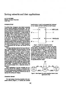
Oct 10, 2014 - less computation steps) than the previously known best networks. There- .... Network Check. Fig. 2. Iterative generation of new inputs. 3 Tools.
Faster Sorting Networks for 17, 19 and 20 Inputs ¨ Thorsten Ehlers and Mike Muller
arXiv:1410.2736v1 [cs.DS] 10 Oct 2014
¨ Informatik, Christian-Albrechts-Universit¨at zu Kiel Institut fur D-24098 Kiel, Germany. {the,mimu}@informatik.uni-kiel.de
Abstract. We present new parallel sorting networks for 17 to 20 inputs. For 17, 19, and 20 inputs these new networks are faster (i.e., they require less computation steps) than the previously known best networks. Therefore, we improve upon the known upper bounds for minimal depth sorting networks on 17, 19, and 20 channels. The networks were obtained using a combination of hand-crafted first layers and a SAT encoding of sorting networks.
1
Introduction
Comparator networks are hardwired circuits consisting of simple gates that sort their inputs. If the output of such a network is sorted for all possible inputs, it is called a sorting network. Sorting networks are an old area of interest, and results concerning their size date back at least to the 50’s of the last century. The size of a comparator network in general can be measured by two different quantities: the total number of comparators involved in the network, or the number of layers the networks consists of. In both cases, finding optimal sorting networks (i.e., of minimal size) is a challenging task even when restricted to few inputs, which was attacked using different methods. For instance, Valsalam and Miikkulainen [11] employed evolutionary algorithms to generate sorting networks with few comparators. Minimal depth sorting networks for up to 16 inputs were constructed by Shapiro (6 and 12 inputs) and Van Voorhis (10 and 16 inputs) in the 60’s and 70’s, and by Schwiebert (9 and 11 inputs) in 2001, who also made use of evolutionary techniques. For a presentation of these networks see Knuth [6, Fig.51]. However, the optimality of the known networks for 11 to 16 channels was only shown recently by Bundala and Z´avodn´y [4], who expressed the existence of a sorting network using less layers in propositional logic and used a SAT solver to show that the resulting formulae are unsatisfiable. Codish, Cruz-Filipe, and SchneiderKamp [5] simplified parts of this approach and independently verified Bundala and Z´avodn´y’s result. For more than 16 channels, not much is known about the minimal depths of sorting networks. Al-Haj Baddar and Batcher [2] exhibit a network sorting 18 inputs using 11 layers, which also provides the best known upper bound on the minimal depth of a sorting network for 17 inputs. The lowest upper bound on the size of minimal depth sorting networks on 19 to 22 channels also stems
from a network presented by Al-Haj Baddar and Batcher [1]. For 23 and more inputs, the best upper bounds to date are established by merging the outputs of smaller sorting networks with Batcher’s odd-even merge [3], which needs dlog ne layers for this merging step. We use the SAT approach by Bundala and Z´avodn´y to synthesize new sorting networks of small depths, and thus provide better upper bounds for 17, 19, and 20 inputs. An overview of the old and new upper bounds as well as the currently best known lower bounds for the minimal depth of sorting networks for up to 20 inputs is presented in Table 1. Table 1. Bounds on the minimal depth of sorting networks for up to 20 inputs.
Inputs 1 2 3 4 5 6 7 8 9 10 11 12 13 14 15 16 17 18 19 20 Old upper bound 0 1 3 3 5 5 6 6 7 7 8 8 9 9 9 9 11 11 12 12 New upper bound 0 1 3 3 5 5 6 6 7 7 8 8 9 9 9 9 10 11 11 11 Lower bound 0 1 3 3 5 5 6 6 7 7 8 8 9 9 9 9 9 9 9 9
2
Our approach
Morgenstein and Schneider [8] and Bundala and Z´avodn´y [4] gave SAT encodings for the search for sorting networks. Using this encoding, the latter authors were able to construct sorting networks as well as prove lower bounds for up to n = 13 input bits. Nevertheless, the running time required by the SAT solver grows exponentially in n. On the one hand, finding sorting networks is known to be NP-complete [10]. On the other hand, their SAT encoding requires O(2n nd) variables for a n-bit sorting network of depth d. Therefore, we show how to reduce the size of the formula in different ways. Reachability Constraints A comparator network is only able to sort all inputs, if there is a directed path from each input pin to each output pin. Using a SAT-encoding of the algorithm of Floyd and Warshall, this fact can be encoded with O(n2 · d) variables. This is, we add more constraints to the SAT formula. Nevertheless, they allow for creating sorting networks without considering all possible input vectors, and hence reduce the overall size of the SAT formula given to the SAT solver. Using Posets for the first layers Parberry [9] showed that if there is a sorting network for n bits with depth d, then there is also one using any maximal first layer, i.e., a layer where no more
comparator may be added. In order to find better sorting networks, one may try and hand-craft more than this one layer. A well-known technique for the creation of sorting networks is the generation of partially ordered sets for parts of the input in the first layers. Figure 1 shows comparator networks which create partially ordered sets for 2, 4 and 8 input bits. In the case of n = 2, the
Fig. 1. Generating partially ordered sets for n ∈ {2, 4, 8} inputs.
output will always be sorted. For n = 4 bits, the set of possible output vectors is given by n �T �T �T �T �T �T o 0000 , 0001 , 0011 , 0101 , 0111 , 1111 , i.e., there are 6 possible outputs. Furthermore, the first output bit will equal zero unless all input bits are set to one, and the last output bit will always be set to one unless all input bits equal zero. Similarly, a poset for n = 8 inputs allows for 20 different output vectors. In order to create faster sorting networks, we heavily used posets in the first layers, and had the other layers created by a SAT solver. Iterative Encoding Knuth observed that a feasible sorting network for n inputs will in particular sort all inputs of the form x = 0a y1b , where a + |y| + b = n and a + b > 0. Bundala and Z´avodn´y found empirically that it is sufficient to consider inputs with less than n unsorted bits to prove lower bounds. We extend this idea, and try to minimize the number of inputs given to the SAT solver. We start with a formula which describes a feasible comparator network satisfying the reachability constraints. This formula is given to a SAT solver. In case there is a satisfying assignment, this result is given to a second SAT solver which is used to compute a counterexample, i.e., an input that cannot be sorted by the network generated by the first solver. If such a counterexample is found, it is added to the formula, and a new comparator network is computed. The process ends if no suitable counterexample can be produced, i.e., the generated comparator network is a feasible sorting network, or no comparator network can be generated which sorts the set of counterexamples generated so far. Interestingly, the combination of necessary constraints for comparator networks to be sorting networks combined with this approach allows for finding proper sorting networks even if only a few different inputs are used.
SAT: Network found
Network Creation
Network Check SAT: Counterexample found
UNSAT: No network found
UNSAT: Network is feasible
Fig. 2. Iterative generation of new inputs
3
Tools
Our software is based on the well-known SAT solver MiniSAT 2.20. Before starting a new loop of our network creation process, we used some probingbased preprocessing techniques [7] as they were quite successful on this kind of SAT formulae.
4
New upper bounds
We present two sorting networks lowering the known upper bounds on the minimal depth of sorting networks. The network presented in Figure 3 is a sorting network for 17 channels using only 10 layers, which outperforms the currently best known network due to Al-Haj Baddar and Batcher [2]. The first three layers are similar to the ones used in the sorting network for 16 inputs and 9 layers from [6]. The remaining layers were created using a SAT solver.
Fig. 3. A sorting network for 17 channels of depth 10.
The network displayed in Figure 4 sorts 20 inputs in 11 parallel steps, which beats the previously fastest network using 12 layers [1]. In the first layer, partially ordered sets of size 2 are created. These are merged to 5 partially ordered sets of size 4 in the second layer. The third layer is used to create partially ordered
sets of size 8 for the lowest and highest wires, respectively. These are merged in the forth layer.
Fig. 4. A sorting network for 20 channels of depth 11.
The wires in the middle of the network are connected in order to totally sort their intermediate output. Using this prefix and the necessary conditions on sorting networks depicted above, we were able to create the remaining layers using our iterative, SAT-based approach. Interestingly, the result was created in 588 iterations, thus 587 different input vectors were sufficient.
References 1. S. W. A. Baddar and K. E. Batcher. A 12-step sorting network for 22 elements. Technical Report 2008-05, Kent State University, Dept. of Computer Science, 2008. 2. S. W. A. Baddar and K. E. Batcher. An 11-step sorting network for 18 elements. Parallel Processing Letters, 19(1):97–103, 2009. 3. K. E. Batcher. Sorting networks and their applications. In American Federation of Information Processing Societies: AFIPS Conference Proceedings: 1968 Spring Joint Computer Conference, Atlantic City, NJ, USA, 30 April - 2 May 1968, volume 32 of AFIPS Conference Proceedings, pages 307–314. Thomson Book Company, Washington D.C., 1968. 4. D. Bundala and J. Z´avodn´y. Optimal sorting networks. In Language and Automata Theory and Applications - 8th International Conference, LATA 2014, Madrid, Spain, March 10-14, 2014. Proceedings, volume 8370 of LNCS, pages 236–247. Springer, 2014. 5. M. Codish, L. Cruz-Filipe, and P. Schneider-Kamp. The quest for optimal sorting networks: Efficient generation of two-layer prefixes. CoRR, abs/1404.0948, 2014. 6. D. E. Knuth. The art of computer programming, volume 3: sorting and searching. Addison-Wesley Professional, 1998.
7. I. Lynce and J. P. M. Silva. Probing-based preprocessing techniques for propositional satisfiability. In 15th IEEE International Conference on Tools with Artificial Intelligence (ICTAI 2003), 3-5 November 2003, Sacramento, California, USA, page 105. IEEE Computer Society, 2003. 8. A. Morgenstern and K. Schneider. Synthesis of parallel sorting networks using SAT solvers. In Methoden und Beschreibungssprachen zur Modellierung und Verifikation von Schaltungen und Systemen (MBMV), Oldenburg, Germany, February 21-23, ¨ Informatik, 2011. 2011, pages 71–80. OFFIS-Institut fur 9. I. Parberry. A computer-assisted optimal depth lower bound for nine-input sorting networks. Mathematical Systems Theory, 24(2):101–116, 1991. 10. I. Parberry. On the computational complexity of optimal sorting network verification. In PARLE ’91: Parallel Architectures and Languages Europe, Vol. I: Parallel Architectures and Algorithms, Eindhoven, The Netherlands, June 10-13, 1991, Proceedings, volume 505 of LNCS, pages 252–269. Springer, 1991. 11. V. K. Valsalam and R. Miikkulainen. Using symmetry and evolutionary search to minimize sorting networks. Journal of Machine Learning Research, 14:303–331, 2013.