FAULT DETECTION AND DIAGNOSIS USING A HYBRID DYNAMIC SIMULATOR: APPLICATION TO INDUSTRIAL RISK PREVENTION Nelly Olivier-Maget, Gilles Hetreux
To cite this version: Nelly Olivier-Maget, Gilles Hetreux. FAULT DETECTION AND DIAGNOSIS USING A HYBRID DYNAMIC SIMULATOR: APPLICATION TO INDUSTRIAL RISK PREVENTION . MOSIM 2014, 10`eme Conf´erence Francophone de Mod´elisation, Optimisation et Simulation, Nov 2014, Nancy, France.
HAL Id: hal-01166664 https://hal.archives-ouvertes.fr/hal-01166664 Submitted on 23 Jun 2015
HAL is a multi-disciplinary open access archive for the deposit and dissemination of scientific research documents, whether they are published or not. The documents may come from teaching and research institutions in France or abroad, or from public or private research centers.
L’archive ouverte pluridisciplinaire HAL, est destin´ee au d´epˆot et `a la diffusion de documents scientifiques de niveau recherche, publi´es ou non, ´emanant des ´etablissements d’enseignement et de recherche fran¸cais ou ´etrangers, des laboratoires publics ou priv´es.
10the International Conference on Modeling, Optimization and Simulation - MOSIM’14 – November 5-7-2014Nancy – France “Toward circular Economy”
FAULT DETECTION AND DIAGNOSIS USING A HYBRID DYNAMIC SIMULATOR: APPLICATION TO INDUSTRIAL RISK PREVENTION
N. OLIVIER-MAGET
G. HETREUX
Laboratoire de Génie Chimique, UMR-5503 (INPT/CNRS/UPS), 4, Allée Emile Monso, BP 84234, F-31432 Toulouse, France
[email protected],
[email protected]
ABSTRACT: The main tool for the development of hazardous chemical syntheses in the field of fine chemicals and pharmaceuticals remains the batch reactor. Nevertheless, even if it offers the required flexibility and versatility, this reactor presents technological limitations. In particular, poor transfer of the heat generated by exothermic chemical reactions is a serious problem with regard to safety. In this context, a simple failure is considered as prejudicial. So, fault detection and diagnosis are studied with a particular attention in the scientific and industrial community. The major idea is that the fault must not be undergone but must be controlled. So, this work presents a fault detection and isolation methodology for the monitoring of Hybrid Dynamic Systems. The developed methodology rests on a mixed approach which combines a model-based method for the fault detection and an approach based on data (pattern matching) for the identification of fault(s). It is integrated within a hybrid dynamic simulator. In this paper, the approach is tested during the operation of an exothermic reaction. The major risk of this system is a cooling failure. The objective of the present work is to detect and diagnosis a fault, before it becomes more serious. In this purpose, two simulations are studied, during which a fault of the material feed and a fault of the energy feed are respectively introduced. KEYWORDS: Fault Detection and Isolation, Extended Kalman Filter, Dynamic Hybrid Simulation, Object Differential Petri Nets Hybrid, Risk assessment
1
INTRODUCTION
Batch and semi-batch processes play an important role in the pharmaceutical and fine chemical process industry. They are the prevalent production modes for low volumes of high added value products. Such systems are characterized not only by a small scale flexible production, but also by complex chemical reaction (Grau et al., 2000). Generally, these processes are complex and not entirely known. For this reason, batch or fed-batch reactors are frequently used for the development of hazardous chemical synthesis. Even if it offers the required flexibility and versatility, this reactor has technological limitations. Particularly, during the exothermic chemical reactions, the poor heat transfer can become a serious safety problem (Stoessel, 2008). Numerous methods of risk analysis such as HAZOP (International standard IEC 61882) can be exploited for the identification of the main events or potentially dangerous deviations. Then, corrective measures can be taken in order to improve the process safety. However, these studies cannot prevent the occurrence of failures during the chemical reaction. For instance, these failures can be due to the malfunction of a sensor or of an actuator. There are also the structural changes, which refer to
changes in the process itself (Venkatasubramanian et al., 2003). These failures occur due to hard failures in equipment, such as a stuck valve, a broken or leaking pipe. Consequently, fault detection and diagnosis are the purpose of a particular attention in the scientific and industrial community. The major idea is that the defect must not be undergone but must be controlled. Nowadays, these subjects remain a large research field. The literature quotes as many fault detection and diagnosis methods as many domains of application (Chang and Chen, 2011; Venkatasubramanian, et al., 2003). A notable number of works has been devoted to fault detection and isolation, and the techniques are generally classified as: - Methods without models such as quantitative process history based methods (neural networks (Venkatasubramanian, et al., 2003), statistical classifiers (Anderson, 1984)), or qualitative process history based methods (expert systems (Venkatasubramanian, et al., 2003)), - Model-based methods which are composed of quantitative model-based methods (such as analytical redundancy (Chow and Willsky, 1984), parity space (Gertler and Singer, 1990), state estimation (Willsky, 1976), or fault detection filter (Franck, 1990)) and qualitative model-based methods (such as causal methods: digraphs
MOSIM’14 – November 5-7-2014 - Nancy - France
(Shih and Lee, 1995), or fault tree (Venkatasubramanian, et al., 2003)). In this paper, the proposed approach to fault detection and isolation is a model-based approach, applied to chemical processes. The first part of this communication focuses on the main fundamental concepts in the field of a batch reactor and of runaway scenarios. Next, the studied reaction is presented. This is the oxidation of sodium thiosulfate with hydrogen peroxide. Then, its protocol is underlined. The third part illustrates the proposed model-based diagnosis approach. It uses the extended Kalman Filter, in order to generate a fault indicator. The high robustness and real-time ability of observer is well-known for industrial applications (Ding, 2014). Next, this approach is enlightened exploited through the simulation of an exothermic reaction monitoring. Finally, section 5 summarizes the contributions and achievements of the paper and some future research works are suggested. 2
-
A level called the Maximum Temperature of the Synthesis Reaction (MTSR) can be reached. At this temperature, a secondary decomposition reaction may be initiated, and the temperature of the mixture increases to reach the final temperature TEND. The runaway reaction can be induced by an increase of the reaction rate (in other words, of the heat production) or by a decrease of the cooling capacity. A heat increase may be initiated either by an increase of the concentrations (causes: feeding, evaporation…), either by a catalytic acceleration (origins: reactive specificities, autocatalysis…), or by a temperature rise (reasons: reaction heat, energy adding). A cooling capacity decrease may come from a decrease of the mixing efficiency (stopping of the stirring motor…), from a decrease of the heat transfer (causes: viscosity increase, etc.), from a quantity or potential increase (for example, due to the use of important quantities), or by a decrease of the power of the cooling system (origins: failures on the cooling system).
EXOTHERMIC CHEMICAL REACTION
The implementation of chemical reactions in batch or semi-batch reactors is strongly limited by the constraints linked to the dissipation of the heat generated by the reactions. Thus, this implementation can be made only after a complete risk analysis has been conducted to guarantee its safety, and the quality of its products (Chetouani et al., 2003). Consequently, we must firstly identify the risk in a chemical reactor. The main risk consists of a runaway scenario. 2.1
Runaway scenario Temperature
TEND Decomposition reaction
2.2
The chosen reaction is a very exothermic oxidoreduction one, the oxidation reaction of sodium thiosulfate Na2S2O3 by hydrogen peroxide H2O2 (Chetouani, 2004). Because of its characteristics, this reaction is particularly exploited for safety study (Xaumier et al., 2002; Chetouani et al., 2003; Prat et al., 2005; Benaissa et al., 2008; Benkouider et al., 2012). The stoechiometric scheme is: Na2S2O3 + 2 H2O2 ½ Na2S3O6 + ½ Na2SO4 + 2 H2O
ΔTad.r
k 0 = 2 ⋅ 1010 L.mol-1.s-1 and Ea = 6.82 ⋅ 104 J.mol-1.
TP Normal process t0
t1
t2
Time
Figure 1: Runaway scenario R. Gygax (1988) proposed the following runaway scenario. He considers the case where a complete cooling failure occurs (Figure 1): - The reactor is initially at the process temperature TP. -
Choice of the reaction
This liquid homogeneous reaction is irreversible, fast, and highly exothermic (Lo and Cholette, 1972). The kinetics can be described by: − Ea r = k ⋅ [Na2 S 2O3 ] ⋅ [H 2O2 ] with k = k0 ⋅ exp (1) R ⋅T
ΔTad.d
MTSR Adiabatic behaviour
The objective of this research work is so to prevent the reaction runaway by detecting the abnormal behaviour and diagnosing the causes of this behaviour.
Next, at t=t0, the cooling stops and so the temperature increases due to the completion of the reaction. This temperature increase depends on the process conditions (Stoessel, 2008).
The reaction heat is ΔHr = -586.2 kJ.mol-1. Some hypotheses are stated: - The reactor is perfectly mixed with a homogeneous temperature in the reaction mixture; -
-
The feeding of the reactive does not induce volume contraction; The heat capacity and the density of pure components are constant in the range of the considered temperatures; The physico-chemical properties of the mixture are constant; The chemical reaction is performed in a pseudohomogeneous medium;
MOSIM’14 – November 5-7-2014 - Nancy - France
-
The thermal losses between the reaction mixture and the ambient surroundings can be neglected.
Na2S2O3 H2O2 H2O Temperature (K) Flowrate (L.h-1)
Weight percent
Material feed 1 15% 75% 293.15 120.9
-
An other feeding step of H2O2 during 1200 seconds, with a constant temperature 333.15 K,
-
A constant temperature step (the reaction step) at 333.15 K during 4800 seconds.
Material feed 2 30% 70% 333.15 31.2
FT2 FC2 Material feed 2
Table 1: Operating Conditions
V2a
The process consists of a standard batch reactor of 100L, connected with a cooling system. The water utility fluid is provided at a temperature of 288.15K. The tank is filled by two material feeds. The aqueous sodium thiosulfate is introduced through the main inlet process fluid. In order to avoid a possible side reaction, H2O2 is in excess. The weight percent in the inlet flows are 15% for Na2S2O3 and 30% for H2O2. The instrumentation of the process is composed of two temperature sensors (mixture and utility fluid), two flow sensors (the reactor feeding flow rate and the utility fluid flow rate). In normal functioning, the operating conditions of a typical oxidation reaction are summarized in Table 1. 2.3
V2b
FT1 Mixer
FC1
Vapour outlet
Material feed 1 V1 Monofluid outlet
V3 Monofluid inlet V4
TT TC
Protocol
TSHH TAH
Figure 2: Semi-batch process A typical operation of a batch or semi-batch reactor consists of the tracking of an a priori defined temperature profile. In the case of an exothermic reaction, three distinct steps are involved: preheating, reaction, and cooling (Xaumier et al., 2002). The reactor temperature is controlled by manipulating the flowrate of the utility fluid. Figure 2 represents the experimental set up used in this study. The process recipe is composed of several steps: - A feeding step of Na2S2O3 during 1200 seconds, -
A heating step to increase the temperature of the mixture from 293.15 K to 333.15 K,
2.4
Risk assessment
The risk management is a major requirement in the industrial context: a major accident is unacceptable. Identifying risks is essential for ensuring the safe design and operation of a process. Several techniques are available to analyse hazardous situations (Marhavilas et al., 2011). Among them, the HAZard and OPerability study (HAZOP) is a well-known technique for studying the hazards of a system (Benaïssa et al., 2008) and its operability problems (International Standard IEC 61882.2001).
Section Guide word
Deviation
Nb
Causes
Reactor More
More flow rate
1
Malfunction of the valves V1a or V2 (for example they remains totally opened)
• • • •
Accumulation of reagents Increase of the reaction speed Increase of the reactor temperature Runaway
2
Malfunction of the controller FC1 or FC2 (for example detection of a wrong value more important)
• • • •
Accumulation of reagents Increase of the reaction speed Increase of the reactor temperature Runaway
3
Malfunction of the valves V1a or V2 : they are closed
• Decrease of the conversion rate • Production loss
4
Plug in pipe
• Decrease of the conversion rate • Production loss
5
Pipe rupture
• Decrease of the conversion rate • Production loss • Big leaks of hazardous product
6
Malfunction of FC1 or FC2: detection of a wrong value (less important)
• Decrease of the conversion rate • Production loss
None
Flow
Table 2: HAZOP data sheet sample
Consequences
MOSIM’14 – November 5-7-2014 - Nancy - France
The HAZOP team studied each element for deviations and considered their undesirable consequences. The identification of deviations is obtained by combining process parameters (temperature, flowrate, pressure…) with “guide words” (no, more, less, as well as, reverse, etc.). Each deviation is studied and particularly we search how undesirable events can occur in order to have this deviation. The conclusions are resumed in a table, (Freeman et al., 1992). Among all the potential hazards highlighted by the HAZOP method, numerous scenarios could potentially lead to a thermal runaway. So, these scenarios were identified as the most hazardous ones. Table 2 illustrates the result data sheet. It gives a short sample of the analysis carried out on the reactor part. 3
FDI METHODOLOGY
Nowadays, for reasons of safety and performance, monitoring and supervision play an important role in process control. The complexity and the size of industrial systems induce an increasing number of process variables and make difficult the work of operators. In this context, a computer aided decision-making tool seems to be wise. Nevertheless the implementation of fault detection and diagnosis for stochastic system remains a challenging task. Various methods have been proposed in different industrial contexts (Venkatasubramanian et al., 2003). The proposed approach is a model-based approach involving the use of Hybrid Dynamic System simulation. 3.1
Architecture
Reference model
– Residual Extended Kalman filter
Process
Signature
+
+
Rebuilt incidence – matrix
Generation of fault indicator
Decision : occurency of fault(s)
For this purpose, the simulation model of PrODHyS is used as a reference model to implement the functions of detection and diagnosis. The supervision module must be able to detect the faults of the physical systems (leak, energy loss, etc.) and the faults of the control/command devices (actuators, sensors, etc.). As defined in (De Kleer et al., 1984), our approach is based on the hypothesis that the reference model is assumed to be correct. The global principle of this system is shown in Figure 3, where the sequence of the different operations is underlined (Olivier-Maget et al., 2008). Moreover, a distinction between the in-line and off-line operations is made. Our approach is composed of three parts: the generation of the residuals, the generation of the signatures and the generation of the fault indicators. This methodology has been the subject of previous studies (Olivier-Maget et al., 2009a, 2009b). Nevertheless, it must be validated with other systems and other fault types, in order to ensure its genericity. Current work aims at extending the application areas of process safety. So, the studied case concerns he implementation of an exothermic reaction. 3.2
Residual generation
The first part concerns the generation of the residuals (waved pattern in the Figure 3). In order to obtain an observer of the physical system, a real-time simulation is done in parallel. So, a complete state of the system will be available at any time. Thus, it is based on the comparison between the predicted behavior obtained thanks to the simulation of the reference model (values of state variables) and the real observed behavior (measurements from the process correlated thanks to the Extended Kalman Filter).
IN LINE OFF LINE
Adjustment of the extended Kalman filter Process and/or faulty simulated system Reference model
+ –
Residual
Incidence matrix: theoretical fault signatures
Experience return
Figure 3: Supervision Architecture The research works performed for several years within the PSE (Process System Engineering) research department of the Chemical Engineering Laboratory of Toulouse on process modelling and simulation have led to the development of PrODHyS (Perret et al., 2004; Hétreux et al., 2007). This environment provides a library of classes dedicated to the hybrid dynamic process simulation. Based on object concepts, PrODHyS offers extensible and reusable software components allowing a rigorous and systematic modelling of processes.
The main idea is to reconstruct the outputs of the system from the measurement and to use the residuals for fault detection (Mehra and Peschon, 1971, Welch and Bishop, 1995, Simani and Fantuzzi, 2006). A lot of state estimators are developed for nonlinear systems (Banerjee and Jana, 2014). Kalman filtering based observer (Li et al., 2004; Qu et Ahn, 2009), extended Luenberger observer (Zeitz, 1987 ; Gundale Mangesh and Jana, 2008), sliding nonlinear observer (Biagiola and Figueroa, 2004; Mezouar et al., 2008), particle filtering (Farza et al., 2004; Olivier et al., 2012) are the most important estimators. The current work focuses on the design of an extended Kalman Filter. A description of the extended Kalman filter can be found in (Olivier-Maget et al., 2008). Besides the residual is defined according to the following equation: Xˆ (t ) − X i (t ) rir (t ) = i with i ∈ {1, n} (2) X i (t ) ˆ is the estimated state where Xi is the state variable, X i
variable with the extended Kalman Filter and n is the number of state variables.
MOSIM’14 – November 5-7-2014 - Nancy - France Note that the generated residual rir (t ) is relative. As a matter of fact, this allows the comparison of residuals of different variables, since the residual becomes independent of the physical size of the variable. 3.3
Signature generation
The second part is the generation of the signatures (doted pattern in the Figure 3). This is the detection stage. It determines the presence or not of a fault. This is made by a simple threshold ε i (t ) . The generated structure S rN i (t ) is denoted by the following equation: S irN
Max rir (t ) − ε'i (t ) ; 0 (t ) = n ∑ Max rkr (t ) − ε'k (t ) ; 0 k =1
with i ∈ {1, n}
(3)
ε (t ) with ε'i (t ) = i , where εi is the detection threshold. X i (t ) The value of ε i is chosen according to the model error covariance matrix of the Extended Kalman Filter (Olivier-Maget, 2007). 3.4
to 1 of these distances. An indicator can be viewed as the probability of the occurrence of a particular fault. Next, these generated indicators are exploited to take a diagnosis of the system. For this, we suppose that: - The minimum value of the indicator, for which the fault can be considered, is 0.68 – chosen according to the normal distribution–. This threshold corresponds to the probability at the standard deviation. -
The number of faults, which can simultaneously take place, is limited to three.
4
RESULTS
The advantage of the simulation of the chemical reaction thermal effect is to prevent runaway problems, which can occur experimentally, particularly for such an exothermic reaction (Xaumier et al., 2002). Then, to demonstrate the good performance of the diagnosis methodology, different simulations have been carried out on the hybrid dynamic simulator PrODHyS. Two faults have been introduced: - Increase of the flow rate (fault 1): In this case, 6500 s after the beginning of the reaction, the feed rate of the sodium thiosulfate is multiplied by 2. -
Generation of fault indicator
The last part deals with the diagnosis of the fault (hatched pattern in the Figure 3). The signature obtained in the previous part is compared with the theoretical fault signatures by means of a distance. A theoretical signature T•,j of a particular fault j is obtained by experiment or in our case, by simulations of the process with different occurence dates of this fault. Then, a fault indicator is generated. For this, two distances have been defined: the relative Manhattan distance and the improved Manhattan distance (Olivier-Maget, 2007). The first distance is denoted by the following expression: n
∑ SirN (t ) − Tij
i =1 D Mr j (t ) =
n
(4)
The second distance, which allows the diagnosis of many simultaneous faults, is denoted by the following expression: n
∑ SirN (t ) × m′ − Tij × n′ ⋅ Tij
i =1 D Ma j (t ) =
(5) n′ where n′ is the number of non-zero elements of the theoretical fault signature T•,j and m′ is the number of
non-zero elements of the fault signature S rN (t ) .
Since both distances are defined in the space interval [0;1], the fault indicators are defined as the complement
4.1
Increase of the jacket temperature (fault 2): 7500 s after the beginning of the reaction, the cooling temperature is increased to 10 °C. Adjustments
To perform a monitoring of a process, some off-line adjustments must be made. On the one hand, we need to determine the covariance matrices of the model and measurement disturbances. While the measurement noises are supposed to be well-known by experiments or by the sensor manufacturer, the model disturbances is estimated by an “ensemble method”. Numerous simulations have been performed during which a model parameter has been disturbed. This allowed the estimation of statistic distribution of the model mistakes. Then, if the behaviour of the system goes beyond this distribution, its behaviour is abnormal. So, the detection thresholds are determined according to the model disturbances. On the other hand, the second adjustment is the learning of the incidence matrix. It is based on the same “ensemble” theory. For this, we perform a set of simulations, during which a fault is introduced at different occurrence dates, for each potential state of the hybrid dynamic system (Figure 4). For this study we consider six faults. These faults are underlined by the HAZOP study. These faults could lead to a thermal runaway: - Fault 1: The material feed 1 provides material with a damaged flow rate; -
Fault 2: The material feed 1 provides material with a damaged composition;
MOSIM’14 – November 5-7-2014 - Nancy - France
-
Fault 4: The material feed 2 provides material with a damaged composition;
-
Fault 5: The energy feed has a damaged temperature;
-
Fault 6: The regulation temperature is damaged. Theoretical signature of the default 0 0.02014515 0 0 0 0 0 0 0.49586922 0 0.48398564
0.6 0.5
s1 s2 s3 s4 s5 s6 s7 s8 s9 s10 s11
Density
0.4 0.3
0.2 0.1
0 s11
s2
s3
s4
s5 s6 s7 Signature
t=0 s t=600 s t=1200 s t=3600 s t=6000 s
s9
s10
Fault 2
Fault 3
Fault 4
Fault 5
0
0
0
0
0
Holdup (mol)
1
0.030239 0.020145
0
0
0
X[Sodium Thiosulfate]
0
0.950786
0
0
0
0
X[Hydrogen Peroxide]
0
0
0
0.289313
0
0.10448
X[Sodium Trithionate]
0
0
0
0
0
0
X[Sodium Sulfate]
0
0
0
0
0
0
X[Water]
0
0.018975
0
0.00103
0
0.000208
Reaction conversion
0
0
0
0
0
Cooling power (W)
0
0 0
Utility flow rate (L/h)
Feed_2
Heat
Reaction
10 9
350
8
300
7 250
6
200
5
150
4 3
100
2 50
1
0
0 0
0.5
1
1.5 2 Time (hours)
2.5
3
3.5
Figure 5: Normal operation
0.495869 0.404899 0.009761 0
0
Detection
s11
0
0
Feed_1
400
4.3 s8
Fault 1
0
Cooling power (kW)
Barycenter
Temperature (K)
0
Holdup (10 x mol)
Molar conversion rate
t=7100 s
For example, figure 4 represents the results obtained for the fault 3. The signatures of this fault are presented for different occurence dates. They have the same pattern. The barycenter is estimated and we obtain the theoretic signature of the fault 3. Next, we perform this preliminary study for all the considered faults of the system and the incidence matrix is presented in table 3.
Fluid Utility Flowrate
Temperature (K)
t=6800 s
Figure 4: Learning of the incidence matrix
Fluid Utility Temperature
highly exothermic. We also notice that the conversion is not total (87%).
Molar conversion rate and Cooling power (kW)
Fault 3: The material feed 2 provides material with a damaged flow rate; Temperature (K), Utility flow rate (L/h) and Holdup (10 x mol)
-
0.049209
0.483986 0.304758 0.94103
Fault 6
0 0.681392 0 0.21392
Let us remind that the thresholds for the detection correspond to the model uncertainties obtained by the adjustment of the Extended Kalman filter. Figure 6 shows the detection step. It illustrates the evolution of the residual linked to the utility fluid flow rate. In order to avoid a false diagnosis, the diagnosis step is not launched as far as the symptoms of the abnormal behaviour appear. The abnormal behaviour is only confirmed after it has occurred three times. Example 1: A fault of the material feed 2 is introduced at t = 6500 s. The material feed 2 provides material with a damaged flow rate (multiplied by 2). From t = 6800 s, the values of the residual underline the abnormal behaviour of the process. The diagnosis is launched at t = 6900 s. Example 2: A fault of the energy feed is introduced at t = 7500 s. The energy feed has a damaged temperature (increasing of 10 °C). From t = 7600 s, the values of the residual underline the abnormal behaviour of the process. The diagnosis is launched at t = 7700 s.
Table 3: Incidence Matrix
4.2
Normal operation
Figure 5 represents the simulated results for a normal operation. It gives the temperature profile of the process mixture, the evolution of the liquid holdup in the reactor, the conversion rate and the characteristics (flow rate and power) of the fluid utility. It must be noticed that the utility fluid flow rate increases during the feeding step of H2O2. It points out that this oxidation reaction is fast and
Residual of the utility fluid flow rate (L/h)
80
Notice that the faults 4 and 6 would be confused, if we work with binary values. The work with real and non binary values aims at distinguishing the importance of the symptoms between a fault with an other one. Therefore, for a particular fault, the normalization allows that the great symptoms are underlined.
Fault 1 Fault 2 60
40
Occurency date of the fault 1
Occurency date of the fault 2
20 Confidence region 0 5000 -20
-40
5500
6000
6500
7000
7500
Detection date of the fault 1
8000
8500
Time (seconds) Detection date of the fault 2
Figure 6: Residual evolution of the utility fluid flow rate
MOSIM’14 – November 5-7-2014 - Nancy - France
Let us notice that the exploited signature in this approach is non binary, in order to quantify the deviation due to the fault. Example 1
Example 2
Temperature (K)
0
0
Holdup (mol)
0.0210
0
X[Sodium Thiosulfate]
0
0
X[Hydrogen Peroxide]
0
0
X[Sodium Trithionate]
0
0
X[Sodium Sulfate]
0
0
X[Water]
0
0
Reaction conversion
0
0
Cooling power (W)
0.5094
0.0007
Fluid Utility Temperature
0
0.1144
Fluid Utility Flowrate
0.4637
0.8849
Table 4: Instantaneous fault signatures of both examples The residual is then estimated and we obtain the corresponding instantaneous fault signature (Table 4). We compare the instantaneous fault signature (Table 4) with the theoretical fault signatures, by calculating the relative and improved Manhattan distances ((3) and (4)). Then, the fault indicators are generated (Table 5). They correspond to the complement to 1 of these distances. Example 1: The relative Manhattan indicator detects the presence of the fault 3 with a probability of 99.68%. Nevertheless, the other faults are not eliminated, since their indicators are higher than 0.68 (cf. the point 3.4). In the opposite, with the improved Manhattan indicator, the faults 1, 2, and 5 are eliminated, since their indicators are lower than 0.68. The three remaining possibilities are the faults 3, 4, and 6. This example underlines the importance of using both indicators to be able to conclude. So, by combining the results of the both indicators, we can rule on the presence of the fault 3, since their indicators are the maximums. For this reason, this fault is the most probable. So, the fault is located on the material feed 2. Furthermore, it has been identified: the material feed 2 provides material with a damaged flowrate. Example 2: The relative Manhattan indicator detects the presence of the fault 5 with a probability of 98.81%. However, none fault is discriminated (all indicators higher than 0,68). With the improved Manhattan indicator, the presence of the fault 5 is distinguished, since the other indicators are lower than 0.68. So, by combining the results of both indicators, we can rule on the presence of the fault 5. Then, the fault is located on the energy feed of the reactor. Furthermore, it has been identified: the cooling energy feed of the reactor has a damaged temperature.
Example 1
Diagnosis
Example 2
4.4
Fault 1
Fault2
Fault 3
Fault 4
Fault 5
Fault 6
Manhattan relative indicator
0.8225
0.8225
0.9968
0.9477
0.9048
0.9502
Manhattan improved indicator
0.0630
0.0954
0.9835
0.8939
0.5435
0.7565
Manhattan relative indicator
0.8182
0.8182
0.9063
0.8737
0.9881
0.8572
Manhattan improved indicator
0
0.0947
0.5600
0.6432
0.9439
0.4289
Table 5: Fault indicators 5
CONCLUSION
In this research work, the feasibility of using the simulation as a tool for fault detection and diagnosis is demonstrated. The fault detection and diagnosis approach, developed here, lies on the hybrid dynamic simulator PrODHyS. It is a general method for the detection and isolation of a fault occurrence. Besides, this approach allows the detection of numerous types of fault and has the ability to underline the simultaneous occurrence of many faults. The works in progress aim at integrating this hybrid dynamic system simulation within a model-based supervision system. The goal is to define a recovery solution following the diagnosis of a default. For this, the results of signatures will be exploited in order to generate qualitative information. For example, with these results, we have the ability to distinguish a simple degradation and a failure. Next, this method will be combined with other diagnosis approaches: the set of the potential faults will be generated according to such methods as classification or case-based reasoning, restricting the search domain (to a part of the process or to a set of potential faults yielding similar symptoms) examined with the model-based technique.. Relating to the operation of exothermic reactions, a novel concept of heat exchangers reactors offers enhanced thermal performances in continuously operating reactors. The experiment results emphasize a significant thermal efficiency: the reactant concentrations and therefore the heat generation can be increased without risk of thermal runaway (Di Miceli Raimondi et al., 2014). The Polysafe ANR project (N° ANR-2012-CDII-0007-01) focuses on the modelling of these reactors in normal and degraded mode, to study the process drift and demonstrate the inherently safer nature of these devices. . REFERENCES Anderson, T.W. (1984). An introduction to multivariate statistical analysis, New York: Wiley. Banerjee S., A. K. Jana, 2014. High gain observer based extended generic model control with application to a
MOSIM’14 – November 5-7-2014 - Nancy - France
reactive distillation column, Journal of Process Control, 24(4), p. 235–248. Benaissa W., N. Gabas, M. Cabassud, D. Carson, S. Elgue, M. Demissy, 2008. Evaluation of an intensified continuous heat-exchanger reactor for inherently safer characteristics, Journal of Loss Prevention in the Process Industries, 21(5), p. 528-536. Benkouider A.M., R. Kessas, A. Yahiaoui, J.C. Buvat, S. Guella, 2012. A hybrid approach to faults detection and diagnosis in batch and semi-batch reactors by using EKF and neural network classifier, Journal of Loss Prevention in the Process Industries, 25(4), p. 694–702. Biagiola S.I., J.L. Figueroa, 2004. A high gain nonlinear observer: application to the control of an unstable nonlinear process, Computers & Chemical Engineering, 28, p. 1881–1898. Chang C.T., C.Y. Chen, 2011. Fault diagnosis with automata generated languages, Computers and Chemical Engineering, 35, p. 329–341. Chetouani, Y., N. Mouhab, J.M. Cosmao and L. Estel, 2003. Dynamic model-based technique for detecting faults in a chemical reaction, Process Safety Progress, 22(3), p. 183-190. Chetouani, Y., 2004. Fault detection by using the innovation signal: application to an exothermic reaction, Chemical Engineering and Processing, 43, p. 1579-1585. Chow, E.Y. and A.S. Willsky, 1984. Analytical redundancy and the design of robust failure detection systems, IEEE Transactions on Automatic Control, 29(7), p. 603-614.
Frank, P.M., 1990. Fault diagnosis in dynamic systems using analytical and knowledge-based redundancy – a survey and some new results, Automatica, 26, p. 459474. Freeman R.A., R. Lee, T.P. McNamara, 1992. Plan HAZOP studies with an expert system, Chemical Engineering Progress, p. 28–32 Gertler, J. and D. Singer, 1990. A new structural framework for parity equation-based failure detection and isolation, Automatica, 26, p.381-388. Grau, M.D., J.M. Nouguès and L. Puigjaner, 2000. Batch and semibatch reactor performance for an exothermic reaction, Chemical Engineering and Processing, 39, p. 141-148. Gundale Mangesh M., A.K. Jana, 2008. A comparison of three sets of DSP algorithms for monitoring the production of ethanol in a fed-batch baker's yeast fermenter, Measurement, 41, p. 970–985. Gygax, R., 1988. Chemical reaction engineering for safety, Chemical reaction engineering for safety, Chemical Engineering Science, 43(8), p. 1759-1771. Hétreux, G., R. Théry, N. Olivier-Maget, J.M. Le Lann, 2007. Exploitation de la simulation dynamique hybride pour la conduite de procédés semi-continus, JESA, 41(5), p. 585-616. Li R., A.B. Corripio, M.A. Henson, M.J. Kurtz, 2004. On-line state and parameter estimation of EPDM polymerization reactors using a hierarchical extended Kalman filter, Journal of Process Control, 14, p. 837– 852.
De Kleer, J. and B.C. Williams, 1987. Diagnosing multiple faults, Artificial Intelligence, 32, p. 97-130.
Lo, S.N. and A. Cholette, 1972. Experimental study on the optimum performance of an adiabatic MT reactor, The Canadian Journal of Chemical Engineering, 50, p. 71-80.
Di Miceli Raimondi N., Olivier-Maget N., Gabas N., Cabassud M., Gourdon C., 2014. Safety enhancement by transposition of the nitration of toluene from semibatch reactor to continuous intensified heat exchanger, Chemical Engineering Research and Design, In Press, Corrected Proof, Available online 9 August 2014.
Mahavilas P.K., Koulouriotis D., Gemeni V., 2011. Risk analysis and assessment methodologies in the work sites: On a review, classification and comparative study of the scientific literature of the period 20002009, Journal of Loss Prevention in the Process Industries, 24(5), p. 477-523
Ding S.X., 2014. Data-driven design of monitoring and diagnosis systems for dynamic processes: A review of subspace technique based schemes and some recent results, Journal of Process Control, 24(2), p. 431– 449.
Mehra, R.K. and J. Peschon, 1971. An Introduction approach to fault detection and diagnosis in dynamic systems, Automatica, 5, p. 637-640.
Farza M., M. M'Saad, L. Rossignol, 2004. Observer design for a class of MIMO nonlinear systems, Automatica, 40, p. 135–143.
Mezouar A., M.K. Fellah, S. Hadjeri, 2008. Adaptive sliding-mode-observer for sensorless induction motor drive using two-time-scale approach, Simulation Modelling Practice and Theory, 16, p. 1323–1336.
MOSIM’14 – November 5-7-2014 - Nancy - France
Olivier B., Huang, I.K. Craig, 2012. Dual particle filters for state and parameter estimation with application to a run-of-mine ore mill, Journal of Process Control, 22, p. 710–717. Olivier-Maget, N., 2007. Surveillance des Systèmes Dynamiques Hybrides : Application aux procédés, PhD Thesis of the Toulouse University (INSA). Olivier-Maget, N., G. Hétreux, J.M. Le Lann and M.V. Le Lann, 2008. Integration of a failure monitoring within a hybrid dynamic simulation environment, Chemical Engineering and Processing, 47(11), p.1942-1952. Olivier-Maget, N., G. Hétreux, J.M. Le Lann and M.V. Le Lann, 2009a. Model-Based Fault Diagnosis Using a Hybrid Dynamic Simulator: Application to a Chemical Process, Computer Aided Chemical Engineering, 27, p. 1641-1646. Olivier-Maget, N., G. Hétreux, J.M. Le Lann and M.V. Le Lann, 2009b. Fault Detection and Diagnosis Based on a Hybrid Dynamic Simulator, published in "The 7th IFAC International Symposium on Fault Detection, Supervision and Safety of Technical Processes", Spain, p. 223-228.
Simani, S. and C. Fantuzzi, 2006. Dynamic system identification and model-based fault diagnosis of an industrial gas turbine prototype, Mechatronics, 16, p. 341-363. Shih, R. and L. Lee, 1995. Use of fuzzy cause-effect digraph for resolution fault diagnosis for process plants, Industrial and Engineering Chemistry Research, 34(5), p. 1688-1717. Stoessel, F., 2008. Thermal safety of chemical processes, Risk assessment and Process Design, Wiley-VCH, p. 374. Venkatasubramanian, V., R. Rengaswamy, K. Yin and S. N. Kavuri, 2003. A review of process fault detection and diagnosis, Computers & Chemical Engineering, 27, p. 293-346. Welch, G. and G. Bishop, 1995. An introduction to the Kalman filter, Technical Report TR 95-041, University of North Carolina. Willsky, A.S., 1976. A survey of design methods for failure detection in dynamic systems, Automatica, 12, p. 601 – 611.
Perret, J., G. Hétreux and J.M. Le Lann, 2004. Integration of an object formalism within a hybrid dynamic simulation environment, Control Engineering Practice, 12(10), p. 1211-1223.
Xaumier, F., M.V. Le Lann, M. Cabassud and G. Casamatta, 2002. Experimental application of nonlinear model predictive control: temperature control of an industrial semi-batch pilot-plant reactor, Journal of Process Control, 12(6), p. 687-693.
Qu C.C., J. Hahn, 2009. Process monitoring and parameter estimation via unscented Kalman filtering, Journal of Loss Prevention in Process Industries, 22, p. 703–709
Zeitz M., 1987. The extended Luenberger observer for nonlinear systems, System & Control Letters, 9, p. 149–156.
Rawlings J.B., B.R. Bakshi, 2006. Particle filtering and moving horizon estimation, Computers & Chemical Engineering, 30, p. 1529–1541.