Noname manuscript No. (will be inserted by the editor)
Fault Oblivious High Performance Computing with Dynamic Task Replication and Substitution Yevgeniy Vorobeychik · Jackson R. Mayo · Robert C. Armstrong · Ronald G. Minnich · Don W. Rudish
Abstract Traditional parallel programming techniques will suffer rapid deterioration of performance scaling with growing platform size, as the work of coping with increasingly frequent failures dominates over useful computation. To address this challenge, we introduce and simulate a novel software architecture that combines a task dependency graph with a substitution graph. The role of the dependency graph is to limit communication and checkpointing and enhance fault tolerance by allowing graph neighbors to exchange data, while the substitution graph promotes fault oblivious computing by allowing a failed task to be substituted on-the-fly by another task, incurring a quantifiable error. We present optimization formulations for trading off substitution errors and other factors such as available system capacity and lowoverlap task partitioning among processors, and demonstrate that these can be approximately solved in real time after some simplifications. Simulation studies of our proposed approach indicate that a substitution network adds considerable resilience and simple enhancements can limit the aggregate substitution errors.
1 Introduction Traditional parallel programming techniques have been developed at platform scales small enough that the various causes of component failure (including hardware, operating system, and application faults) can be neglected to a first approximation. Thus the emphasis has been on optimizing application performance under a rare-failure assumption, and separately on ensuring sufficient levels of component reliability to comply with this assumption. In common paralYevgeniy Vorobeychik · Jackson R. Mayo · Robert C. Armstrong · Ronald G. Minnich · Don W. Rudish Sandia National Laboratories, P.O. Box 969, Livermore, CA 945510969, USA E-mail:
[email protected]
lel programming models such as MPI, an entire parallel job halts if a single component contributing to the job fails, and so an add-on mechanism is required to deal with failures if one or more of them are likely to occur during a job. The “checkpoint-restart” solution, where a snapshot of the global state of the application is periodically saved to disk and used to resume the job in the event of failure, enables long jobs to run to completion at a manageable cost in additional computing time, but only when failures are sufficiently rare – more precisely, when the system-wide mean time between failures (MTBF) is large compared to the time required to save a checkpoint [4]. Continuing large increases in system size, without corresponding increases in MTBF for individual components, are reducing the system-wide MTBF for leading HPC platforms to levels where checkpoint-restart will not remain practical. As the system-wide MTBF becomes smaller than the checkpointing time, forward progress of traditionally designed applications will slow dramatically and their useful completion will become effectively impossible; thus the benefits of exascale computing will not be fully realized in such a framework. Various enhancements, such as predictive monitoring to checkpoint selectively when failure is more likely [2], can extend the feasibility of checkpoint-restart to a degree, but by themselves are expected to be insufficient for exascale computing. We introduce a software architecture, based on a largely decentralized use of dependency and substitution graphs, that promotes a high degree of fault tolerance and even fault obliviousness. While task dependency graphs have a long history in parallel computing, our suggested use of them in conjuction with task substitution graphs is novel. The architecture is general, but allows considerable flexibility in responding to failures of computation nodes if a job has appropriate structure. Specifically, we take advantage of two kinds of structure: (a) sparse dependencies among tasks and (b) similarity of computation products of different tasks. The
2
Yevgeniy Vorobeychik et al.
former is encoded in a dependency graph, while the latter motivates the substitution graph. The key idea is that if a task fails and a close substitute is still available, we can dynamically remap the dependency without having to restart the entire job or even the failed task. Furthermore, we can quantify how much error in results is introduced by substitutions, allowing a principled tradeoff between substitutions and task restarts. We implement our architecture in simulation and demonstrate its efficacy and resilience, showing in addition that we can limit substitution errors as well as developer burden by using simple empirical techniques to derive substitution weights.
2 Example Application Before presenting our architecture for fault oblivious computing, it will be useful to keep in mind a specific application. Our application of choice is distributed asynchronous value iteration, which we subsequently use to test our approach in simulation. Value iteration is one of the algorithms for computing the values of states of a discounted Markov decision process (MDP) [7]. An MDP evolves over a sequence of discrete time steps, proceeding through a series of states belonging to a set S. At a fixed time step t, the decision maker finds himself in some state st ∈ S, and must choose some action at ∈ A(st ), where A(st ) is the set of feasible actions in state st . Upon taking action at in state st , he receives a probabilistic reward rt and probabilistically transitions to the next state st+1 . The Markovian property ensures that both the distribution over rewards and the distribution over next states depend only on the current state and action. We consider a slightly simplified model in which rewards are a deterministic function of current state; thus, rt = r(st ). We denote the distribution over next states by P, with Pssa 0 meaning the probability of transitioning from state s to s0 if action a is taken in state s. A solution to an MDP is a policy π, which determines the sequence of action choices as a function of state, denoted π(s). An optimal policy π ∗ is the policy that maximizes the expected reward with a discount factor δ , that is, ∞
π ∗ = arg max ∑ δ t E[r(st )|π]. π
The corresponding expected reward (value) of any state s ∈ S is V ∗ (s), which can be alternatively expressed by the Bellman equation [7]:
∑ Pssa 0 V ∗ (s0 ).
Vn+1 (s) = r(s) + δ max
∑ Pssa 0 Vn (s0 ).
(3)
a∈A(s) s0
This algorithm is provably convergent to the true vector of valuations V ∗ . Moving from a serial to a parallel implementation of the value iteration algorithm is rather natural. For simplicity, suppose that a processor is tasked with computing a value for a single state s ∈ S (thereby eschewing any state partitioning issues for the moment). The internal data on the processor will be r(s), δ , and the part of Pssa 0 with s as the initial state, which can be represented as a matrix with a as rows, s0 as columns, and corresponding transition probabilities as entries. At each iteration, the entire vector Vn must be broadcast to all processors in order to compute Vn+1 [1]. There are three problems with this approach: 1. it requires synchronization, with the concomitant performance cost; 2. it requires broadcast transmission of the entire vector Vn in every iteration n; and 3. it requires internally storing data of size |S||A(s)|. The most important issue is the second, since message passing is likely the performance bottleneck and, with large state spaces, the parallel algorithm will become entirely impractical as a consequence (message passing will dominate computation). Synchronization is the easiest issue to overcome in a natural way: Rather than requiring all states to broadcast their values Vn synchronously, let them do so every time a new value is computed. In this way, each state has the latest vector of values, but the process no longer requires any synchronization. It turns out that asynchrony does not preclude convergence, as long as processors do not stall (i.e., values of all states keep being updated) [6]. The other two issues are resolved by the decentralized dependency graph, described below.
3 Dependency and Substitution (DAS) Architecture for Dynamic Task Replication and Substitution
(1)
t=0
V ∗ (s) = r(s) + δ max
the Bellman equation. At iteration n, the value Vn+1 (s) is computed as
(2)
a∈A(s) s0
Value iteration [1,7] is a natural algorithm for iteratively computing optimal state values V ∗ that stems directly from
The goal of this section is to introduce a general architecture that allows effective failure management and, under some conditions, fault obliviousness in exascale computing scenarios. Here, we envision jobs that are divided into a very large number of interdependent tasks. Consequently, a failure of one processor running a certain task can potentially bring down the entire job due to the intricate interdependencies. Our goal is to manage such interdependencies in order to dynamically restart tasks or replace them with other tasks that generate similar data. To this end, we introduce two
Fault Oblivious High Performance Computing with Dynamic Task Replication and Substitution
a
b c
d
Fig. 1 Example of a simple dependency graph involving four tasks.
graphical data structures: a dependency graph and a substitution graph. The former keeps track of data dependencies between tasks, while the latter is a representation of substitution relationships between tasks (that is, whether data from one task can substitute for the data from another, possibly failed, task). The former structure primarily manages failures, while the latter is a means of fault obliviousness, insofar as it can be achieved. As the architecture depends on these two graphical structures, we term it the DAS (dependency and substitution) architecture.
3.1 Dependency Graph A dependency graph is a directed graph representation of data dependencies between tasks, with each node representing a computational task (e.g., computing the value of a state s), while a directed edge from i to j means that task i depends on task j (for example, a non-zero probability transition from s to s0 ). Figure 1 shows a simple example. In parallel computing, we wish to decentralize information as much as possible, and so it would be greatly undesirable (if not entirely impractical) to maintain a completely centralized dependency graph. Instead, each node maintains the dependency subgraph immediately relevant to it. In our simulated implementation, a node merely maintains the list of all nodes that it depends on, as well as those nodes that depend on it, although a more robust implementation would allow it also to maintain dependencies of its inputs (i.e., of the nodes it depends on), etc. The first thing that a decentralized dependency graph gains us is a simple resolution of the scalability issues outlined in our discussion of value iteration in Section 2 (but applicable broadly). In our case, rather than broadcast messages being sent to all nodes, a node queries all its dependencies for their values via message passing, limiting communication to a potentially small fraction of the tasks at any given time. Observe that a dependency graph is completely general, since it allows all tasks to be interdependent, but its benefits arise only if it is sparse. Focusing now on our stated main task of fault tolerance and obliviousness, the dependency graph provides our main mechanism for fault tolerance. Suppose that a task i detects that one of its dependencies j has failed (perhaps because j did not respond to some query within a timeout period, or i was notified of this failure either by the failing node or by the operating system). If i already has the requisite data from
3
j, it needs to do nothing. If not, it can notify the system of the failure. If there is a provision in the running job to restart specified tasks, or if there is a checkpoint that we can refer back to, the failed task can again be placed on the run queue to be restarted so as to provide the needed data to i. Note that we do not require that the dependency graph be specified at the time that the main job is started; it can be generated dynamically, as tasks are spawned by the main process. An important aspect is the decentralization of the graph, so that tasks themselves may determine whether any failed dependency actually needs restarting. Consider, for example, a situation in which a task that fails is not depended upon by any other task. Its failure will then go essentially unnoticed, except, perhaps, by the system, and so the job may well continue running, entirely oblivious to any failure having occurred. This ensures that progress can be made even in the presence of frequent node failures. Another utility of the dependency graph is that it can be a means of restoring state without frequent checkpointing. Checkpointing is known to be extremely expensive, often dominating performance, and reducing the frequency of checkpointing can account for dramatic performance improvement. Now, suppose that computation of a task produces incremental results, which also provide a starting point at the time of restart. If these incremental (intermediate) results of a computation are multicast to those tasks that depend on it, then in the event of a task failure and restart, the task can receive these intermediate results from its dependencies without requiring any checkpointing (except, perhaps, the checkpoint required to start up the task at all). As a result, checkpointing can be infrequent. While such “hotstarts” are not yet a part of our implementation, they could provide an important part of the proposed architecture without very much added effort. The dependency graph is a key data structure that allows us to implement decentralized fault tolerance and, to some degree, fault obliviousness. The key data structure that targets specifically fault obliviousness (to the extent it is possible) is the substitution graph, which we turn to next. 3.2 Substitution Graph A substitution graph specifies, for node i, a collection of nodes that generate data that can substitute for the data generated by i, as well as weights for each representing the upper bound on loss (error) incurred due to substitution. As an example, consider a pair of states in value iteration that transition to each other with high probability for some actions, and suppose that the discount factor is not too low. The values at these two states are natural substitutes, since each state can be reached from the other in a single step. While it is not necessary that substitution relationships are reciprocal, it is quite natural that they are, and we therefore
4
Yevgeniy Vorobeychik et al.
0.1 a
b 0.2
0.01 c
0.05
d
Fig. 2 An example of a simple substitution graph involving four tasks. Numbers above edges represent weights on substitutions, that is, errors incurred due to these substitutions.
(rather than replicated), and let zi jk denote a decision to substitute task j for i for a dependent task k (thereby replacing k’s dependence on i with j). We then obtain the following mixed integer program (MIP): max ∑ vi v,z
subject to:
Error budget: assume that the substitution graph is undirected. An example of a substitution graph is shown in Figure 2. Note that while it seems also natural that the substitution relationships are transitive, they need not be. To see why transitivity may fail, note that it is only meaningful to include edges between tasks that can substitute at some relatively small loss, i.e., loss below some fixed threshold. Thus, it could be that a sequence of tasks can substitute for each other with relatively small error, but once the length of that sequence is long enough, the substitution error between its endpoints may accumulate to exceed the threshold, and the endpoints would thus be missing an edge even though they are connected by a path. Transitivity would obtain, however, if substitution errors are zero along such a path. The substitution graph mediates fault obliviousness as follows. Suppose that a processor (and a corresponding task) fails, but there is a good substitute for this task (in terms of generated data). The tasks that depend on it may then use the best substitute, rather than requiring the failed task to be restarted. In many domains, the closeness of two tasks would depend on who is using the results. If we implement the substitution graph in a decentralized fashion, as we do in our simulations, allowing for this is a trivial generalization, since each node then simply stores internally its private set of substitution weights together with the sets of substitutes for the tasks it depends on.
3.3 Trading Off Replication and Substitution The main operation of the DAS architecture is to trade off replication and substitution by attempting to substitute for tasks as long as it is efficacious to do so. Specifically, suppose that we set an upper bound ε on the acceptable error for the job. Let us first consider a simplification where, when failures occur, we take a myopic point of view that no further failures will occur before the conclusion of the entire job. We now introduce some formal notation that will allow us to pose the tradeoff we wish to address as a mixed integer program. First, suppose that all errors are additive (e.g., using the l1 norm). Let wi jk be the error incurred when task j is substituted for task i as input to a task k that depends on i. Let I be the set of tasks that have failed and Di denote the set of tasks that depend on a task i ∈ I. We denote by vi a decision variable that is 1 if task i is to be substituted for
(4)
i∈I
∑ ∑ ∑ wi jk zi jk ≤ ε,
(5)
∑zi jk = vi ∀i ∈ I, k ∈ Di ,
(6)
zi jk = 0 ∀i, j ∈ I, k ∈ Di ,
(7)
i∈I j∈I / k∈Di
Single substitute for i, j:
j∈I /
No failed tasks: Binary variables:
vi ,zi jk ∈ {0, 1}.
(8)
Note that constraint (7) is actually unnecessary to specify in practice, since we can simply ignore the corresponding entries of z in implementing the optimal policy; constraint (6) already ensures that there is exactly one substitute from only the functioning tasks for any task dependency pair if and only if the corresponding vi = 1. While the number of variables and constraints is polynomial, solving this integer program is likely infeasible in many realistic cases. To allow us to make the tradeoff in real time, consider the following simpler program. Denote by Ni the number of tasks that depend on i (and that will be using the substitute). Restrict attention to wi j without reference to k (or maximal over all k); then focus only on best substitutes for any failed i, letting wi = Ni min j∈I / wi j , and allow only a single substitute for any task. This results in the following MIP: max ∑ vi v
subject to:
(9)
i∈I
error budget:
∑wi vi ≤ ε,
(10)
vi ∈ {0, 1}.
(11)
i∈I
binary variables:
Observe that the resulting MIP represents a classic knapsack problem, which, while NP-hard, can be approximated by a greedy algorithm that adds tasks to be substituted in increasing order of wi , until the error budget is saturated. This greedy heuristic would be fast enough to be run in real time and is, in fact, what we implemented in our simulations.
3.4 Empirical Substitution Weights The central as yet unanswered question relating to the substitution graph is how to obtain the substitution weights. One possibility is that they are given (as upper bounds, perhaps, or some crude approximation) by the job developer himself, who knows something about the relationship between tasks. That may be reasonable in some scenarios, but would usually place a high burden upon the programmer. A simple alternative is to derive them empirically.
Fault Oblivious High Performance Computing with Dynamic Task Replication and Substitution
Suppose that each task generates data over time that can be represented as a sequence of real vectors. Given such sequences for two tasks that are meant to substitute for each other, we can create an empirical measure of the substitution weight as the observed distance between the generated data streams according to some predefined distance metric. For example, if the error between the entire data streams is important, we could use Hausdorff distance between the two sequences, while if only the latest updates are significant, it would suffice to measure, say, l1 distance between the latest data generated (as is the case in our grid world example below). We may still wish for the programmer to specify the actual substitution weights, as well as initial weights, but neither is strictly speaking necessary: We can measure weights between pairs of tasks, and add a substitution edge if the empirical weight is below some threshold (or, instead, place a threshold on the number of edges, and only add those with the lowest empirical weight). If the programmer does not specify initial weights, we can take them to be infinite by default, forcing replication until sufficient data about tasks are obtained to make substitutions useful. 3.5 Allocating Tasks to Processors In the discussion above, we have implicitly assumed that a single task is allocated to a processor. This is also a very explicit assumption in the simulations below. Although we have not lost much generality by this assumption in our discussion, we now wish to address explicitly the situation in which multiple tasks are allocated to a single processor. The question of interest in our framework becomes two-fold: (a) how to allocate tasks to processors so that there is minimal interdependence between processors and (b) how to substitute in a way that preserves this initially low interdependence. To begin, let us assume that no substitution is allowed. In this case, our problem is an instance of graph partitioning [5]. In a graph partitioning, the goal is to partition a set of nodes in a graph such that the weighted sum of nodes in each partition is bounded by some positive integer K and the weighted sum of edges between partitions is bounded by another positive integer J. This problem is known to be NP-complete, although fast algorithms to solve it exist, including in the Zoltan library [3]. In our case, all weights would be 1. To incorporate information about substitutes, we can superimpose the two graphs and choose weights on substitute edges to be lower than those on dependency edges (to reflect that we may not need to substitute at all). Additionally, weights may decay as the substitution weights wi jk increase. To preserve low processor interdependence during task substitution decisions, we can add a graph partitioning constraint on substitutions when tasks fail, requiring that, upon
5
substitution, no more than J dependencies cross processor boundaries. Formally, letting p jk = 1 if and only if tasks j and k run on different processors, we constrain that
∑∑
p jk zi jk ≤ J
∀i ∈ I
(12)
j∈I / k∈Di
in the first MIP above. In the second, simplified, MIP, let pik = 1 if and only if the best substitutes for tasks i and k lie on different processors. We then constrain that
∑
pik vi ≤ J
∀i ∈ I.
(13)
k∈Di
Note, however, that adding the latter constraint means that we can no longer apply the simple greedy algorithm as described above, and alternative, custom heuristics would need to be developed.
3.6 Running Tasks with a Limited Number of Processors One important subproblem when resources are severely constrained is to determine whether it is possible to run a subset of tasks on available processors, given a specified dependency graph. Specifically, suppose that there are not enough processors to run the entire job. In principle, if all tasks are interdependent, it may be impossible to make any progress until all tasks can be allocated concurrently. However, if dependencies are sparse, it may still be feasible to make progress on the problem by running a subset of tasks that is independent of any others. It turns out that this problem can be solved in polynomial time by the following algorithm (assuming that each task is mapped to a single processor): 1. Let T be the set of all tasks, K the number of available processors 2. For each task i ∈ T , – Let D = Di – For each j ∈ D, – set D ← D ∪ D j – until D j ⊂ D ∀ j ∈ D – If |D| ≤ K, return D 3. return 0 The running time of this algorithm is O(n3 ), where n is the number of tasks, and it will return either a set of tasks D with no external dependencies satisfying |D| ≤ K, or 0 if such a set cannot be constructed. Furthermore, the asymptotic running time falls to O(n2 ) if the number of dependencies between tasks is bounded by a constant. Since we follow the dependency links from all possible starting points (all tasks), this algorithm is complete. The problem is that even though it runs in quadratic time if the maximum number of dependencies is bounded by a constant, this is still too slow to do in real time in an exascale computing system. A possible solution is to perform the
6
Yevgeniy Vorobeychik et al.
!"#
!"#$ !"%$ !"&$ !"'$ !"&$ !"($
%&!"#
!"#$ !"&$ !"($
Fig. 3 Example of a 3 × 3 grid world with the corresponding state reward structure.
procedure only until we run out of search time (perhaps on a random permutation of tasks) in the outer loop, and only for a small number of iterations of the inner loop.
'()*$+&
!"#$%&
!$# Fig. 4 The 2-state Markov chain model of the processor failure and repair process.
or V (s0 ) −V (s) ≤ V (s0 )(1 − δ Pssa 0 )
4 Simulation and Results
for any action a, and, simultaneously,
We use simulations to provide a limited evaluation of our DAS architecture, implemented in Java. These are centered on the application to distributed asynchronous implementation of value iteration in the domain of a “grid world”, which we now describe.
V (s0 ) ≥ δ Psa0 sV (s)
4.1 The Grid World The grid world is a simple geographical representation of an agent walking in two dimensions. In our even simpler representation, an agent is allowed at most four actions in each cell: left, right, up, and down (corresponding essentially to the directions of a walk). The catch is that a walk to the right does not necessarily result in the agent ending up in the cell immediately to the right. Rather, he moves in the direction of his action with probability p (0.8 in our implementation), while the remaining probability is divided evenly among all the remaining physically adjacent cells, as well as the current cell. The rewards of states are generated independently following a distribution with Pr{r(s) ≤ r} = r1/3 . Figure 3 shows an example 3 × 3 grid world, where the number in each cell indicates the reward received by an agent for visiting it. In our implementation, we set the discount factor δ to be 0.95, and let the number of states vary, while maintaining the square shape of the grid. To prevent computation from proceeding indefinitely, we also set a stopping criterion to be convergence within 0.001. Based on the grid world model, we generate the dependency graph by adding links in both directions between any two neighboring cells. Since neighboring cells also provide good substitutes for each other, we add links between all neighbors in the substitution graph. Initial or default weights are generated as upper bounds on the difference between final state valuations. These differences can be bounded by observing that, if s and s0 are neighbors, then V (s) ≥ δ Pssa 0 V (s0 )
(14)
%&!$#
0
(15)
(16)
or V (s) −V (s0 ) ≤ V (s)(1 − δ Psa0 s )
(17)
for any a0 . Taking a and a0 to maximize the right-hand side in Equations (14) and (16), we get the tightest bounds. This is the case when the action in the grid world is toward s0 and s respectively, which achieves the fixed transition probability p that an agent ends up in the direction he tried to follow. Further, if δ is the discount factor, then V (s) ≤ 1/(1 − δ ) for any state s. Combining, we get |V (s) −V (s0 )| ≤
1−δ p . 1−δ
(18)
Note that if p is large, the difference between values of neighbor cells is tightly bounded, while with a small p, this bound is loose. In any case, this provides either the actual or initial substitution weights in our simulations (actual if we turn off empirical tuning of substitution weights, and initial if we turn it on).
4.2 Simulation Setup To perform a first-order analysis of the proposed architecture, we developed simulation software that generates sample grid worlds and performs asynchronous distributed value iteration, with the architecture governing how tasks are allocated computing time on a simulated cluster. Time in the simulator is discrete, and we run it for 100 iterations (time units). Given the high discount factor, this ensures that tasks rarely complete in the allotted time, even if no processor failures occur. We assume, furthermore, that processors fail independently with probability pb , and a broken processor is fixed with probability p f . Figure 4 shows the resulting Markov chain process that models transitions between fixed and broken states for each processor. Given these parameters
Fault Oblivious High Performance Computing with Dynamic Task Replication and Substitution -."/01/2302.4/"
of a Markov chain, which is clearly ergodic and aperiodic, a natural question is what characterizes its steady state. Letting π f and πb be the steady state probabilities of being in the fixed and broken states respectively, it turns out that
As a consequence, we observe that the main parameter that governs the fraction of time each processor spends in a fixed or broken state (and, thus, the expected number of fixed and broken processors) is α = p f /pb . For example, setting α = 1 ensures that 1/2 of all processors are functional on average in the steady state. In the simulation, we let the number of processors be twice the number of tasks, and set α = 1, thereby focusing primarily on the variance due to a specified failure probability (since, on average, there are enough processors to run all the tasks, but often in reality there will not be). Furthermore, we initialize the processors to be in a broken or fixed state precisely according to the corresponding steady state fractions. Our choice that the steady state fraction of available processors matches exactly the number of tasks that need solving may seem idiosyncratic, since it is easy to ensure that we have enough tasks such that they are not prone to processor failures (and, thus, at most we only require replication, but not substitution of tasks). Note, however, that we in general wish to utilize all the available resources: For example, if we choose to discretize a problem more coarsely purely due to system considerations, we would be wasting available system capacity, which is certainly undesirable. Furthermore, such simplifications introduce error into our problem, which we can potentially avoid by fully utilizing available processing capacity. Thus, we would actually expect that the system capacity is (nearly) fully utilized, at least at peak time.
4.3 Performance Measures In our simulations, we evaluate two extreme policies; the first allows no substitutions at all, whereas the second allows unlimited substitution. Thus, neither policy actually involves solving the optimization problems described above, and our results are in a sense unfavorable, since it is quite likely that in fact a mix of replication and substitution is necessary for good performance. The first performance measure is the probability that the tasks make any progress in a given iteration (note that since all the tasks in the grid world example are initially interdependent, either all or none can make progress, depending on processor availability). The second performance measure is the l1 error (relative to failure-free runs) of the computed state values.
!#'"
!"#$"%&"'(()*
(19)
54678739:"/01/2302.4/"
("
!#&"
!#%"
!#$"
!" !"
!#("
!#$"
!#)"
!#%"
!#*"
!#&"
!#+"
!#'"
!#,"
("
!"#+,-./"')*
Fig. 5 Probability that tasks are making progress on a 10 × 10 grid world as a function of failure probability (with α = 1). -."/01/2302.4/"
54678739:"/01/2302.4/"
("
!#'"
!"#$"%&"'(()*
πf pf = . πb pb
7
!#&"
!#%"
!#$"
!" !"
!#("
!#$"
!#)"
!#%"
!#*"
!#&"
!#+"
!#'"
!#,"
("
!"#+,-./"')*
Fig. 6 Probability that tasks are making progress on a 50 × 50 grid world as a function of failure probability (with α = 1).
4.4 Simulation Results We ran simulations with two problem instances, one with 100 tasks, the other with 2500. While both are a far cry from the exascale environment that we target, they allow us to focus on the primary issues that concern us: resilience in the face of frequent failures and scalability, at least to a limited degree. The results we present are averaged over 150 random realizations of the grid world model. Our initial inquiry concerns the first performance measure: probability that any progress is made in a given iteration. Figures 5 and 6 plot the probability of making any progress on a 10 × 10 and 50 × 50 grid, comparing a case where no substitutions are allowed with one that allows unlimited substitutions. These figures strongly demonstrate the increased resilience of the jobs due to the substitution framework: With arbitrary and unlimited substitutions, the failure probability has to approach 1 before progress is even somewhat halted. By comparison, the progress ratio drops dramatically with increasing failure probability when no substitutions are allowed. Considering now the l1 error measure, our results are somewhat mixed (see Figures 7 and 8). On a 10 × 10 grid, it
8
Yevgeniy Vorobeychik et al. -."/01/2302.4/"
54678739:"/01/2302.4/"
;01/3"