Such large point population leads to a high computational cost while doing the fusion in 3D space. Therefore, we introduce a feature-based unsupervised.
FEATURE-BASED FUSION OF TOMOSAR POINT CLOUDS FROM MULTIVIEW TerraSAR-X DATA STACKS Yuanyuan Wang(1), Xiao Xiang Zhu(1,2) (1) Lehrstuhl für Methodik der Fernerkundung, Technische Universität München, Arcisstraße 21, 80333 Munich, Germany (2) Remote Sensing Technology Institute (IMF), German Aerospace Center (DLR), Oberpfaffenhofen, 82234 Weßling, Germany ABSTRACT This article presents a technique of fusing point clouds from multiple view angles generated using synthetic aperture radar (SAR) tomography. Using TerraSAR-X high resolution spotlight data stacks, one such point has a population of about 2×10⁷ points, with a density of around 106 points / km2. Such large point population leads to a high computational cost while doing the fusion in 3D space. Therefore, we introduce a feature-based unsupervised technique for point clouds fusion by detecting and matching building contour end points and aligning flat roofs in the two point clouds. The same idea can also be exploited as a general way to evaluate the fusion accuracy of other fusion techniques. Index Terms— SAR, SAR Tomography, PSI, urban monitoring 1. INTRODUCTION Very high resolution SAR tomography (TomoSAR) enables us for the first time to generate point clouds of a city from space with a point density comparable to LiDAR. The density of one such point cloud we generate is around 106 points / km2. However, due to the side-looking geometry of SAR, these point clouds are different from those generated by LiDAR. In the TomoSAR point cloud, information is rich on the building façades facing the sensor. Therefore, data from different view angles are required to be fused together in order to create a complete point cloud of the area. Previous research on similar fusion task has been carried out in [1] for point clouds generated by persistent scatterer interferometry (PSI). The fusion is done by matching ground point pairs using cross correlation, random sample consensus (RANSAC), and least square adjustment. In [2], the same technique was applied to TomoSAR point
clouds. Because of the layover separation capability and no pre-selection of pixels, a TomoSAR point cloud is usually much denser (around 10 times) than a PSI point cloud. However, the fusion was done by using only the best 10% of the ground points in the point clouds. In order to maximally exploit the rich information of building façades in TomoSAR point clouds for fusion, we choose a quick unsupervised approach that horizontally finds the best completeness of building contours and vertically aligns mean heights of flat planes, rather than matching only the ground point pairs. It consists of three main steps: (1) façade extraction, (2) building L-shape end points detection and matching, and (3) horizontal plane detection and matching. 2. TOMOSAR POINT CLOUD GENERATIO 2.1. Fusion procedures The TomoSAR processing aims at separating multiple scatterers layovered in the same pixel, and retrieving their third coordinate elevation in the SAR native coordinate system. Usually, the images in the stack were acquired at different times, so the displacement of the scatterers must also be modeled and estimated. This is commonly known as differential SAR tomography (D-TomoSAR) [3]-[5]. We use DLR’s TomoSAR software Tomo-GENESIS ([5] [6]) to process TerraSAR-X data stacks of different view angles. For an input data stack, the Tomo-GENESIS retrieves the following information: the number of scatterers inside a pixel, amplitude and phase, topography and motion parameters (e.g. linear deformation velocity and amplitude of thermal dilation induced seasonal motion) of each detected scatterer. After geocoding, a raw 3D point cloud with attributes of motion parameters is obtained. 2.2. Point cloud filtering using k nearest neighbors Such a raw 3D point cloud contains points with a wide range of quality, because of the high dynamic range of
signal-to-noise ratio (SNR) in a SAR image whose square root is inversely proportional to the Cramér-Rao lower bound of the elevation estimates. Figure 1(a) is an example of a raw TomoSAR point cloud. The height of the points is color coded, with blue referring to low and red to high. Therefore, point cloud filtering is necessary to eliminate the outliers. Commonly, they are elevated away from the nearby major 3D structures. Following this, the filtering is done by setting a threshold on each point of the mean distance to its k nearest neighbors (kNN). Such filter is very effective against “lonely” points (see Figure 1(b)), but will fail when encounter a large cluster of outlier points.
(a)
selected points using RANSAC; (3) instead of counting all the points in the black box, only points whose projections in x-y plane within a certain distance to the green dashed line are considered in the point density computation. During the density estimation, particular attention is put on the end points of façades. For points close to the façade ends, the effective area in the directional window is computed by finding the largest cluster and the area it occupies in the window. Figure 3 is the point density result of a test area near Berlin central station. The building contours could already be identified. The façade points will then be selected by thresholding on the density.
(b)
Figure 1. (a) Raw point cloud of Berlin central station, and (b) filtered point cloud. Color represents the height.
3. POINT CLOUDS FUSION The most common TomoSAR point clouds fusion task is to match two from ascending and descending orbits (sensor looking towards east and west). Such two point clouds do not share any common points on building façades but only ground points. Therefore in [1], fusion is done by matching only the ground points. The fusion procedures explained below also applies to this scenario.
Figure 2. Comparison of directional and box-car façade filter. The colored points are the 2D projection of the 3D point cloud, with the color indicating the point density. The green dashed line segment is a robust fit to the 2D projection in a selected area. Points within the region bounded by the solid green lines are considered in the directional point density estimation, while those within the black box are considered in the box-car density estimation. 5
3.1. Façade extraction by directional filter 4
To detect the building contour, façade points must be firstly extracted. Because of the vertical accumulation of these points, the point density on a façade is usually higher than other areas. The most straightforward approach to obtain the point density is using a moving box, and counting the point density in the box. Here we use a directional filter considering the direction of the façade. This approach can eliminate the influence from the ground points, and fill up possible gaps between segments of the same façade in the density estimation.
3 2 1 0 2
The point density estimation for a target point projected on the x-y plane is illustrated in Figure 2. It consists of three steps: (1) all the points are projected to the x-y plane; then an area is selected centered at the target point (the red dot); (2) a straight line segment (the green dashed line) passing through the target point is fitted to the
Figure 3. Point density [points/m ] of a test area near Berlin central station.
3.2. Building segmentation To make the detection of the contour of individual building easier, in this step, the whole point cloud is segmented to building blocks. The building layer extracted
from OpenStreetMap (showing in Figure 4(a)) is used to label each building, as shown in Figure 4(b). The color is randomly assigned to represent different building segments.
Flat roofs are indicated by the low variance in the vertical direction (i.e. z direction). The variance in z direction is simply estimated by taking into account the points within a box around the target point. After detecting many clusters of flat roofs, their centers in x-y plane and mean heights are calculated by simple averaging. 3.5. End points and roof heights matching
(a)
(b)
Figure 4. (a) Building shape layer extracted from OpenStreetMap, and (b) segmented building blocks. Color is segment number which is randomly assigned.
3.3. L-shape detection L-shape is the most common building outline appearing in TomoSAR point clouds. For each building segment, one or zero L-shape is detected. The detection is achieved by catching two interconnected line segment using gray-scale Hough transform [7]. Each pixel in the Hough transform matrix represents a line. In our algorithm, the pixel with the highest amplitude is firstly extracted, representing the first line of the L-shape. The second one is the pixel with highest amplitude away from the first one larger than a certain angle. To reject irregular L-shapes, constraints have to be put on this angle, the minimum pixel amplitude, and the minimum length of the line segments. For example, Figure 5 is the L-shape detection result of the test area near the Berlin central station. The detected Lshapes are overlaid on the binary façade image. The end points of L-shapes are marked with red and yellow dots.
Before the matching of L-shapes end points and mean roof height, an initial rough alignment of these two point cloud is performed using the cross correlation of the projections in x-y, y-z, and z-x plane. As a result, the potential end point pairs and roof center pairs should be closely spaced in the two point clouds. With such prior knowledge, RANSAC is used to find the reliable point pairs. The final shift vector is obtained by a least square adjustment of the detected end points pairs, and roof center pairs, respectively. Figure 6 shows the matched L-shapes from the ascending and descending point cloud. Incomplete L-shape is allowed, if the same L-shape is detected in both point clouds. In our test area, a total 150 pairs of end points are detected, giving a shift of [0.51 -0.09 0.00] in the x, y, z direction. Such shift vector could also be an indication of the fusion accuracy of the roughly fused point clouds. Therefore, our proposed method can be used as a quick blind evaluation of fusion quality when no ground truth is available.
Figure 6. Matched L-shapes, and their end points. Incomplete L-shapes are also allowed, if the same L-shape is detected in both point clouds. (a)
(b)
Figure 5. Detected L-shapes from (a) the ascending and (b) the descending stack overlaid on the gray-scale point density image. The red dots mark the end points of the L-shapes, and the yellow dots are the vertexes.
3.4. Flat roof detection and matching
4. CONCLUSION This paper describes a sequence of procedures to generate a complete high resolution 3D city point cloud from TerraSAR-X data stacks of multiple view angles. TomoSAR inversion is applied to each data stack, estimating the 3D location of the scatterers in the scene.
Results from different data stacks are fused to generate a complete one. Particular focus of this paper is put on the fusion of the point clouds. The fusion is done in a feature-based approach. Firstly façade points from each stack are extracted by thresholding the point density that is estimated for each grid point in x-y plane using a directional filter by taking into account the façade orientation. The output is a rough building outline. Secondly, individual building blocks are found out using the building shape layer extracted from OpenStreetMap. Then, L-shape detection is performed on each of these building blocks using a gray-scale Hough transform. The corresponding end points of the detected L-shapes are identified. In this step, flat roof points are also detected by simple thresholding on the variance of vertical direction. Lastly, end points and roof centers from different point clouds are matched. 5. ACKNOWLEDGMENT This work is supported by the project 6.08: “4D City” of International Graduate School of Science and Engineering (IGSSE), Technische Universität München (TUM). The authors gratefully acknowledge the Gauss Centre for Supercomputing e.V. (www.gauss-centre.eu) for funding this project by providing computing time on the GCS Supercomputer SuperMUC at Leibniz Supercomputing Centre (LRZ, www.lrz.de).
6. REFERENCES [1] S. Gernhardt, X. Cong, M. Eineder, S. Hinz, R. Bamler, “Geometrical Fusion of Multitrack PS Point Clouds”, IEEE Geoscience and Remote Sensing Letters 9(1), pp. 38-42 [2] Y. Wang, X. Zhu, Y. Shi., R. Bamler, “Operational TomoSAR Processing Using TerraSAR-X High Resolution Spotlight Stacks from Multiple View Angles”, In proceedings of IGARSS, Munich, Germany, 2012. [3] F. Lombardini, “Differential Tomography: A New Framework for SAR Interferometry”, In proceedings of IGARSS, Toulouse, France, pp.1206–1208, 2003. [4] G. Fornaro, D. Reale, F. Serafino, “Four-Dimensional SAR Imaging for Height Estimation and Monitoring of Single and Double Scatterers”, IEEE Transactions on Geoscience and Remote Sensing 47(1), pp: 224 – 237, 2009. [5] X. Zhu, R. Bamler, “Very High Resolution Spaceborne SAR Tomography in Urban Environment”, IEEE Transactions on Geoscience and Remote Sensing 48(12), pp. 4296 – 4308 [6] X. Zhu, R. Bamler, Let's Do the Time Warp: MultiComponent Nonlinear Motion Estimation in Differential SAR Tomography, IEEE Geoscience and Remote Sensing Letters 8(4), pp.735-739. [7] R. Lo, W. Tsai, “Gray-scale Hough Transform for Thick Line Detection in Gray-scale Images”, Pattern Recognition 28 (1996) 647–661. [8] N. Adam, B. Kampes, M. Eineder, J.Worawattanamateekul, and M. Kircher, “The Development of A Scientific Permanent Scatterer System”, In processdings of ISPRS Hannover Workshop, Hannover, Germany, 6–8 October, pp. 1–6 (on CD-ROM).
Figure 7. Fusion of two point clouds generated from TerraSAR-X data stacks of ascending and descending orbit. The color represents the height.